4.3 The Histogram: a graph for quantitative variables

The histogram presents continuous (quantitative) data by dividing the variable into equally sized groups, called bins. Histograms allow you to see the spread and shape of the data and get a sense of the center. Is the data normally distributed, or does it have a left or right skew? (There is more about univariate statistics in chapter 5 and more about histograms here

ggplot automatically selects 30 bins. You can adjust this by selecting the number of bins (bins =) or selecting the width of the bins (binwidth =). Mostly ggplot does a good job. No adjustments will be needed.

ggplot(data = my_usstate_data_2011_small) + geom_histogram(mapping = aes(x = pctfemaleleg)) +
  ggtitle("Percentage of Women in State Legislatures, 2011") +
  labs(x = "variable = Percentage Women", y = "Number of States", caption = "Source: ICPPR State Data") +
  theme_minimal()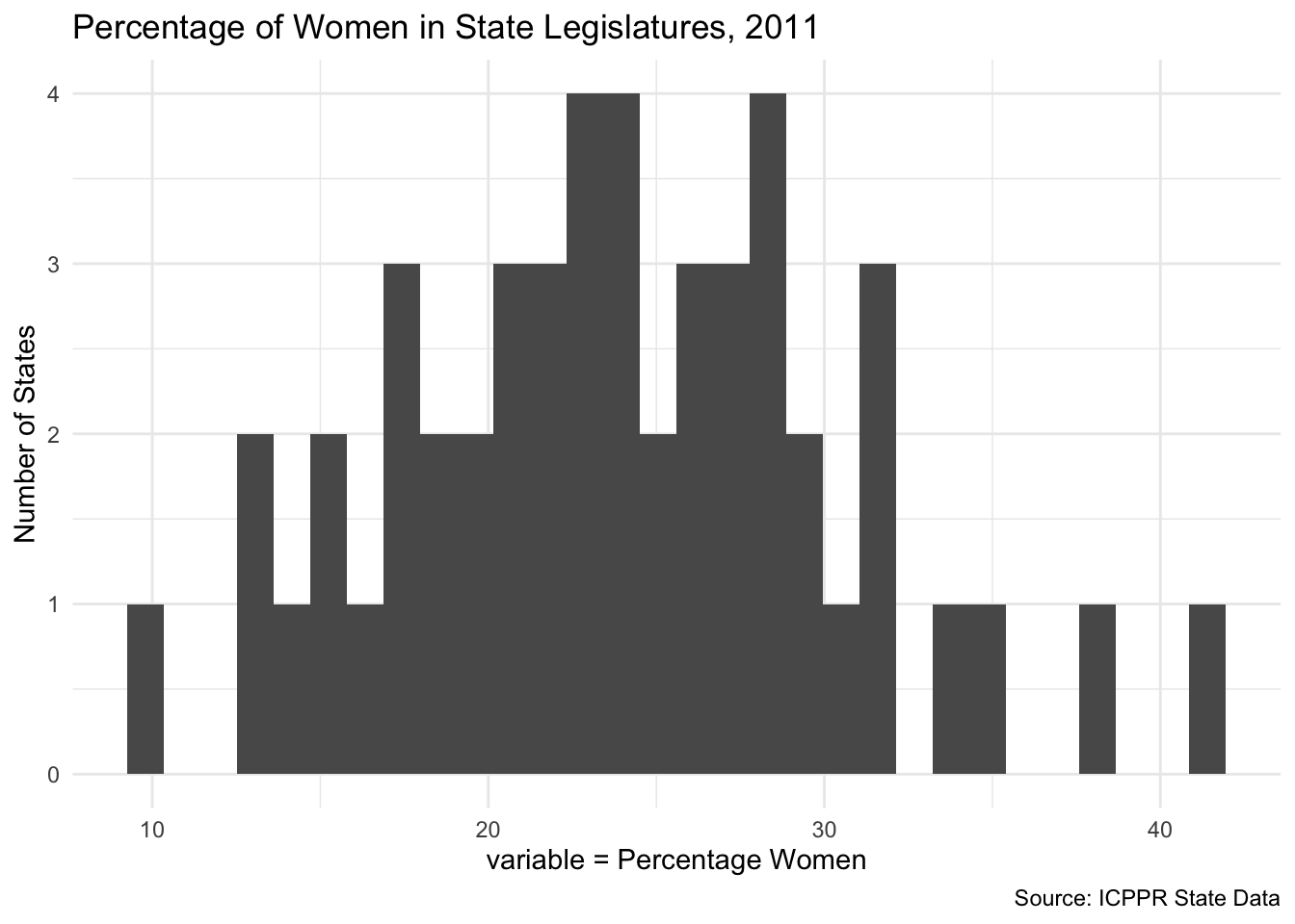

ggplot(data = my_gapminder_data_2003) + geom_histogram(mapping = aes(x = co2EmissionsPerPerson)) +
  ggtitle("CO2 Emissions per Country, 2003") +
  labs(x = "variable = co2EmissionsPerPerson", y = "Number of Countries", caption = "Source: Gapminder")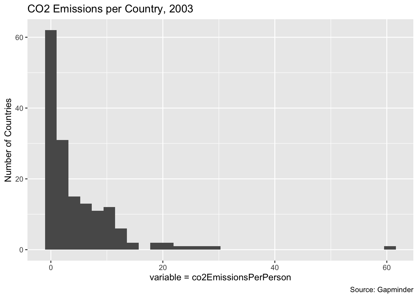

The first of these graphs use state-level data and looks at the percentage of women in state legislatures. The second graph looks at CO2 emissions per person in countries. Note that the state data has close to a normal distribution, but the CO2 emissions graph has a significant right-skew.