8.2 Chi-Square

Chi-square uses categorical variables. For this example, we will use Example 1 from Chapter 7.2 that examines the relationship between education and perception of human rights in Ethiopia. You can look at the original example here.

We can now run our chi-square test. The general model looks like this (and remember you can copy this text):

by(dataset, dataset$3rdVariable, function(x)
   list(chisq.test(x$dependentVariable, x$independentVariable),
        chisq.test(x$dependentVariable, x$independentVariable)$observed,
        prop.table(chisq.test(x$dependentVariable, x$independentVariable)$observed,2)))

And for our example, we will run the chi-square test.

by(ethiopia_small, ethiopia_small$Q260, function(x)
  list(chisq.test(x$Q253, x$Q275R),
       chisq.test(x$Q253, x$Q275R)$observed,
       prop.table(chisq.test(x$Q253, x$Q275R)$observed,2)))

## ethiopia_small$Q260: Male
## [[1]]
## 
##  Pearson's Chi-squared test
## 
## data:  x$Q253 and x$Q275R
## X-squared = 11.054, df = 6, p-value = 0.08671
## 
## 
## [[2]]
##                          x$Q275R
## x$Q253                    Lower Middle Higher
##   A great deal of respect    63     10     17
##   Fairly much  respect      141     48     38
##   Not much respect          108     38     34
##   No respect at all          65     36     21
## 
## [[3]]
##                          x$Q275R
## x$Q253                         Lower     Middle     Higher
##   A great deal of respect 0.16710875 0.07575758 0.15454545
##   Fairly much  respect    0.37400531 0.36363636 0.34545455
##   Not much respect        0.28647215 0.28787879 0.30909091
##   No respect at all       0.17241379 0.27272727 0.19090909
## 
## ------------------------------------------------------------ 
## ethiopia_small$Q260: Female
## [[1]]
## 
##  Pearson's Chi-squared test
## 
## data:  x$Q253 and x$Q275R
## X-squared = 5.2522, df = 6, p-value = 0.5119
## 
## 
## [[2]]
##                          x$Q275R
## x$Q253                    Lower Middle Higher
##   A great deal of respect    61      9      8
##   Fairly much  respect      167     41     30
##   Not much respect          125     42     22
##   No respect at all          58     17     10
## 
## [[3]]
##                          x$Q275R
## x$Q253                         Lower     Middle     Higher
##   A great deal of respect 0.14841849 0.08256881 0.11428571
##   Fairly much  respect    0.40632603 0.37614679 0.42857143
##   Not much respect        0.30413625 0.38532110 0.31428571
##   No respect at all       0.14111922 0.15596330 0.14285714

In looking at the p-values we see that for males it is .087, for females the p-value is .512. Neither meets the required value of less than .05 to be statistically significant. We cannot reject the null hypothesis in either case. We would also want to interpret the tables as well.

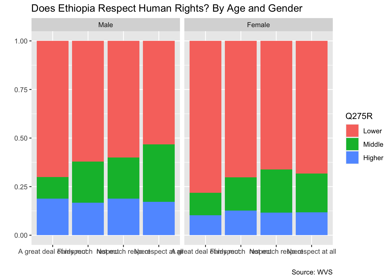
8.2.1 Representing this model in a faceted bar plot

To represent these three variables in a graph, we need to add one line to our two-variable graph, facet_wrap(), adding the third variable. Don’t forget the tilde ~. (Note: This variable needs additional work because the variable is age groups, but the model is appropriate for your work.)

ethiopia_small %>%
  filter(!is.na(Q253)) %>%
  filter(!is.na(Q275R)) %>%
  ggplot(aes(x = Q253, 
             fill = Q275R)) + 
  geom_bar(position = "fill") +
  ggtitle("Does Ethiopia Respect Human Rights? By Age and Gender") +
  labs(x = "", y = "", caption = "Source: WVS") +
  facet_wrap(~ Q260)