6.1 Bar Graphs: C -> C, Q -> C, C -> Q
6.1.1 If your categorical dependent (response) variable has two categories
For this first example, we want to look at the relationship between town size and literacy. I hypothesize that Ethiopians living in larger towns are more likely to be literate. Let’s begin by looking at the frequencies of the two variables.
## Frequencies
## ethiopia_small$E1_LITERACY
## Label: Respondent´s literacy
## Type: Factor
##
##                    Freq   % Valid   % Valid Cum.   % Total   % Total Cum.
## ---------------- ------ --------- -------------- --------- --------------
##         Literate    826     67.15          67.15     67.15          67.15
##       Illiterate    404     32.85         100.00     32.85         100.00
##             <NA>      0                               0.00         100.00
## Total 1230 100.00 100.00 100.00 100.00## Frequencies
## ethiopia_small$G_TOWNSIZE2
## Label: Settlement size_5 groups
## Type: Factor
##
## Freq % Valid % Valid Cum. % Total % Total Cum.
## --------------------- ------ --------- -------------- --------- --------------
## Under 5,000 196 15.93 15.93 15.93 15.93
## 5000-20000 645 52.44 68.37 52.44 68.37
## 20000-100000 357 29.02 97.40 29.02 97.40
## 100000-500000 23 1.87 99.27 1.87 99.27
## 500000 and more 9 0.73 100.00 0.73 100.00
## <NA> 0 0.00 100.00
## Total 1230 100.00 100.00 100.00 100.00My dependent variable is literacy. It is a categorical variable with two categories. For now, the town categories work well. (We might consider whether we should combine the categories for the two largest towns since they both have few respondents.)
Below is our initial graph. As discussed in the PDS video, we are graphing the percentage of our dependent variable (literacy, E1_LITERACY) in each of the independent variable categories (town size, G_TOWNSIZE2). Note: We are using a different graph than noted in PDS Video #7.
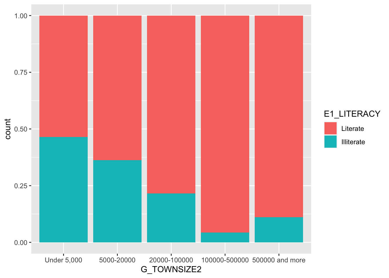
This basic graph is easy to interpret. In small towns, just over 50 percent of the respondents are literate. This percentage goes up for each category except the last, towns with over 500,000 people. (Remember there are few respondents in these categories.)
This basic plot works fine, but we will make two changes for readability. We will:
- Add axis labels and a title.
- Use a theme to make for a better appearance. We will use the built-in
theme_minimaltheme. https://ggplot2.tidyverse.org/reference/ggtheme.html If you are willing to install fonts onto your computer https://github.com/hrbrmstr/hrbrthemes
ggplot(ethiopia_small,
       aes(x = G_TOWNSIZE2,
           fill = E1_LITERACY)) +
geom_bar(position = "fill") +
ggtitle("Ethiopian Literacy Rate by Population of Town") +
labs(x = "Population of Town", y = "Proportion Literate", caption = "World Values Survey, Wave 7") +
theme_minimal()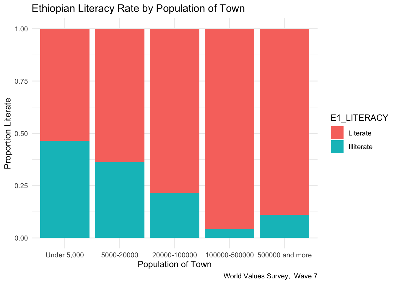

6.1.2 If your categorical dependent (response) variable has more than two categories
For our next example, I want to see whether Ethiopian’s views on whether their country respects individual human rights depend on whether the respondent lives in an urban or rural environment. I hypothesize that people living in larger towns will be more likely to say that Ethiopia respects human rights. Attitude on human rights (Q253) is our dependent variable. Let’s look at the frequency.
## Frequencies
## ethiopia_small$Q253
## Label: Respect for individual human rights nowadays
## Type: Factor
##
##                                 Freq   % Valid   % Valid Cum.   % Total   % Total Cum.
## ----------------------------- ------ --------- -------------- --------- --------------
##       A great deal of respect    169     13.91          13.91     13.74          13.74
##          Fairly much  respect    468     38.52          52.43     38.05          51.79
##              Not much respect    371     30.53          82.96     30.16          81.95
##             No respect at all    207     17.04         100.00     16.83          98.78
##                          <NA>     15                               1.22         100.00
##                         Total   1230    100.00         100.00    100.00         100.00
I have gone ahead and added the title, axis labels, a caption, and a simpler theme.
ethiopia_small %>%
  filter(!is.na(Q253)) %>%
  ggplot(aes(x = H_URBRURAL,
           fill = Q253)) +
  geom_bar(position = "fill") +
  labs(y = "Proportion") +
  ggtitle("Ethiopia Respect for Human Rights by Population of Town") +
  labs(x = "Urban or Rural?", y = "Proportion Think that Ethiopia Respects Human Rights", caption = "World Values Survey,  Wave 7") +
  theme_minimal()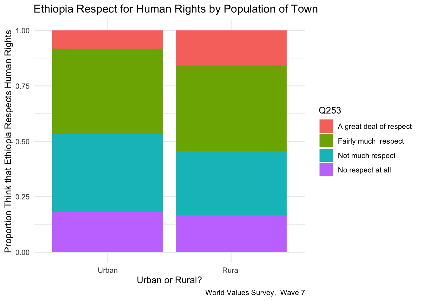
## Cross-Tabulation, Row Proportions
## Q253 * H_URBRURAL
## Data Frame: ethiopia_small
## Label: filelabel
##
## ------------------------- ------------ ------------- ------------- ---------------
##                             H_URBRURAL         Urban         Rural           Total
##                      Q253
##   A great deal of respect                 24 (14.2%)   145 (85.8%)    169 (100.0%)
##      Fairly much  respect                113 (24.1%)   355 (75.9%)    468 (100.0%)
##          Not much respect                104 (28.0%)   267 (72.0%)    371 (100.0%)
##         No respect at all                 54 (26.1%)   153 (73.9%)    207 (100.0%)
##                      <NA>                  1 ( 6.7%)    14 (93.3%)     15 (100.0%)
##                     Total                296 (24.1%)   934 (75.9%)   1230 (100.0%)
## ------------------------- ------------ ------------- ------------- ---------------
This graph is more complicated than one with two variables. Stacked bars can be tricky to interpret. It is often helpful to produce a table as well. (We will talk more about continengy tables in the next chapter.) It looks like there is a difference between urban and rural Ethiopians. Rural Ethiopians being more likely to think that their country respects human rights than urban Ethiopians.
6.1.3 Recoding your categorical independent (explanatory) variable so that it has fewer categories
Let’s return to our first example and reexamine the relationship between town size and literacy. I hypothesized that Ethiopians living in larger towns are more likely to be literate. Let’s begin by again looking at the frequencies of the two variables.
## Frequencies
## ethiopia_small$E1_LITERACY
## Label: Respondent´s literacy
## Type: Factor
##
##                    Freq   % Valid   % Valid Cum.   % Total   % Total Cum.
## ---------------- ------ --------- -------------- --------- --------------
##         Literate    826     67.15          67.15     67.15          67.15
##       Illiterate    404     32.85         100.00     32.85         100.00
##             <NA>      0                               0.00         100.00
## Total 1230 100.00 100.00 100.00 100.00## Frequencies
## ethiopia_small$G_TOWNSIZE2
## Label: Settlement size_5 groups
## Type: Factor
##
## Freq % Valid % Valid Cum. % Total % Total Cum.
## --------------------- ------ --------- -------------- --------- --------------
## Under 5,000 196 15.93 15.93 15.93 15.93
## 5000-20000 645 52.44 68.37 52.44 68.37
## 20000-100000 357 29.02 97.40 29.02 97.40
## 100000-500000 23 1.87 99.27 1.87 99.27
## 500000 and more 9 0.73 100.00 0.73 100.00
## <NA> 0 0.00 100.00
## Total 1230 100.00 100.00 100.00 100.00In looking at our independent variable, town size (G_TOWNSIZE2), we may want to simplify the graph by collapsing categories. The categories for “100000-500000” people and “500000 and more” people each have few respondents, let’s combine them. We will use fct_collapse command in the forcats package to do this. Note: forcats is part of the tidyverse.) We recode and clean up the value labels.
ethiopia_small$G_TOWNSIZE2_recode <- fct_collapse(ethiopia_small$G_TOWNSIZE2,
   "Under 5,000" = c("Under 5,000"),
   "5000-20000" = c("5000-20000"),
   "20000-100000" = c("20000-100000"),
   "100000 and more" = c("100000-500000", "500000 and more"),
)

freq(ethiopia_small$G_TOWNSIZE2_recode)
## Frequencies
## ethiopia_small$G_TOWNSIZE2_recode
## Label: Settlement size_5 groups
## Type: Factor
##
## Freq % Valid % Valid Cum. % Total % Total Cum.
## --------------------- ------ --------- -------------- --------- --------------
## Under 5,000 196 15.93 15.93 15.93 15.93
## 5000-20000 645 52.44 68.37 52.44 68.37
## 20000-100000 357 29.02 97.40 29.02 97.40
## 100000 and more 32 2.60 100.00 2.60 100.00
## <NA> 0 0.00 100.00
## Total 1230 100.00 100.00 100.00 100.00ggplot(ethiopia_small,
aes(x = G_TOWNSIZE2_recode,
fill = E1_LITERACY)) +
geom_bar(position = "fill") +
ggtitle("Ethiopian Literacy Rate by Population of Town") +
labs(x = "Population of Town", y = "Proportion Literate", caption = "World Values Survey, Wave 7") +
theme_minimal()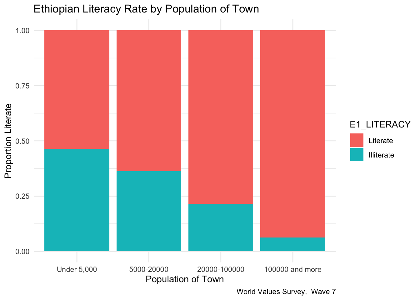
We see a notable increase in literacy by town size. In small communities, the literacy rate is about 55%, while in cities of 100,000 or more people, the literacy rate is about 85%.
6.1.4 Creating a bar chart with a quantitative dependent (response) variable
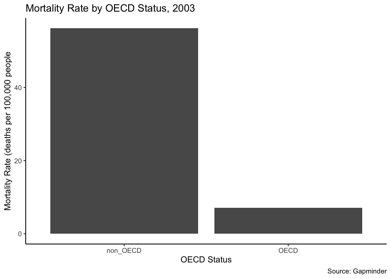
One final example. I want to explore if mortality rates are higher in non-OECD countries than in OECD countries. I hypothesize that they are. The two variables that can help us examine this in the Gapminder dataset, g77_and_oecd_countries and mortalityRate. mortalityRate is a quantitative variable. g77_and_oecd_countries is a categorical variable. Let’s look at the frequencies to see if the variable needs to be recoded.
## Frequencies
## my_gapminder_data_2003$g77_and_oecd_countries
## Type: Character
##
##                Freq   % Valid   % Valid Cum.   % Total   % Total Cum.
## ------------ ------ --------- -------------- --------- --------------
##          g77    102     67.55          67.55     62.58          62.58
##         oecd     28     18.54          86.09     17.18          79.75
##       others     21     13.91         100.00     12.88          92.64
##         <NA>     12                               7.36         100.00
##        Total    163    100.00         100.00    100.00         100.00
There are three categories, “g77” (a large group of developing countries), and “other” in addition to OECD countries (democracies with the largest economies). We need to recode to create two categories, OECD and non-OECD. Because this variable is coded with names, and not numbers, we change the names directly and these can also serve as variable labels.
my_gapminder_data_2003$g77_and_oecd_countries_recode <- fct_collapse(my_gapminder_data_2003$g77_and_oecd_countries,
        "OECD" = c("oecd"),
        "non_OECD" = c("g77", "others")
          )
Finally, we will create the graph. We are doing several things in this code:
- NAs are filtered out.
- The graph shows the mortality rate on the y-axis.
- A title, a caption, and axis labels are added.
- We use a new theme,
theme_classic.
my_gapminder_data_2003 %>%
  filter(!is.na(g77_and_oecd_countries_recode)) %>%
  ggplot() +
  stat_summary(mapping = aes(x = g77_and_oecd_countries_recode, y = mortalityRate), fun= "mean", geom = "bar")  +
  ggtitle("Mortality Rate by OECD Status, 2003") +
  labs(x = "OECD Status", y = "Mortality Rate (deaths per 100,000 people", caption = "Source: Gapminder") +
  theme_classic()