8.3 Correlation

We will use Example 2 in Section 7.3 to examine the potential moderating effect of a third variable. The model looks at the impact of a nation’s GPD on a nation’s life expectancy. We will see if the continent has a moderating effect.

In running a correlation test for a third variable, we need a categorical variable. Continent is already a categorical variable, so we don’t need to do any data management here.

The general format for the third, moderating, correlation test is (and remember you can copy this text):

by(dataset, dataset$3rdVariable, function(x)
  cor.test(x$dependentVariable, x$independentVariable))

Run a correlation test between GDP per capita and life expectancy for each of the five continents.

by(gapminder, gapminder$continent, function(x)
  cor.test(x$lifeExp, x$gdpPercap))

## gapminder$continent: Africa
## 
##  Pearson's product-moment correlation
## 
## data:  x$lifeExp and x$gdpPercap
## t = 11.73, df = 622, p-value < 2.2e-16
## alternative hypothesis: true correlation is not equal to 0
## 95 percent confidence interval:
##  0.3591151 0.4878012
## sample estimates:
##       cor 
## 0.4256076 
## 
## ------------------------------------------------------------ 
## gapminder$continent: Americas
## 
##  Pearson's product-moment correlation
## 
## data:  x$lifeExp and x$gdpPercap
## t = 11.619, df = 298, p-value < 2.2e-16
## alternative hypothesis: true correlation is not equal to 0
## 95 percent confidence interval:
##  0.4751696 0.6316663
## sample estimates:
##       cor 
## 0.5583655 
## 
## ------------------------------------------------------------ 
## gapminder$continent: Asia
## 
##  Pearson's product-moment correlation
## 
## data:  x$lifeExp and x$gdpPercap
## t = 8.2059, df = 394, p-value = 3.287e-15
## alternative hypothesis: true correlation is not equal to 0
## 95 percent confidence interval:
##  0.2945926 0.4631563
## sample estimates:
##       cor 
## 0.3820476 
## 
## ------------------------------------------------------------ 
## gapminder$continent: Europe
## 
##  Pearson's product-moment correlation
## 
## data:  x$lifeExp and x$gdpPercap
## t = 23.644, df = 358, p-value < 2.2e-16
## alternative hypothesis: true correlation is not equal to 0
## 95 percent confidence interval:
##  0.7368907 0.8181201
## sample estimates:
##       cor 
## 0.7807831 
## 
## ------------------------------------------------------------ 
## gapminder$continent: Oceania
## 
##  Pearson's product-moment correlation
## 
## data:  x$lifeExp and x$gdpPercap
## t = 15.373, df = 22, p-value = 2.992e-13
## alternative hypothesis: true correlation is not equal to 0
## 95 percent confidence interval:
##  0.9005401 0.9812620
## sample estimates:
##       cor 
## 0.9564738

The table below summarized the correlations and p-values.

Continent	Correlation	p-value
Africa	.425	2.2e-16
Americas	.558	2.2e-16
Asia	.382	3.287e-15
Europe	.781	2.2e-16
Oceania	.956	2.992e-13

This data shows a strong positive correlation and a strategically significant relationship between GPD per capita and life expectancy for each of the five world regions.

8.3.1 Representing this model in a scatterplot

We will represent this relationship with a scatterplot. There are two good options for representing all three variables in ggplot. One is to use color to represent the third variable. The second is to create multiple graphs, called facets in ggplot, as we did for representing the models we used in ANOVA and chi-square.

First, we’ll look at using color. We do this by adding the color command in the aesthetics. We identify the variable to be used. In this case we add color = continent.

ggplot(data = gapminder) + geom_point(mapping = aes(x= log(gdpPercap), y = lifeExp, color = continent)) +
  ggtitle("Life Expectancy by Per Capita GDP and Continent, 2008") +
  labs(x = "Log of Per Capita GDP", y = "Life Expectancy in Years", caption = "Source: Gapminder", color = "Continent") +
  theme_bw()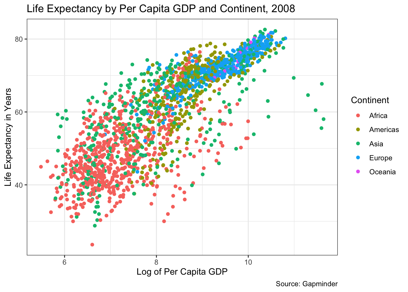

An alternative is to use faceting. We do this by using the facet_wrap command, which is added as the last line below.

ggplot(data = gapminder) + geom_point(mapping = aes(x= log(gdpPercap), y = lifeExp)) +
  theme_bw() +
  ggtitle("Life Expectancy by Per Capita GDP and Continent, 2008") +
  labs(x = "Log of Per Capita GDP", y = "Life Expectancy in Years", caption = "Source: Gapminder") +
  facet_wrap(~ continent)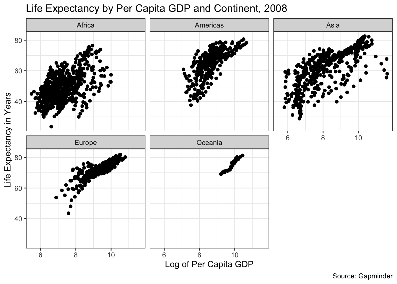

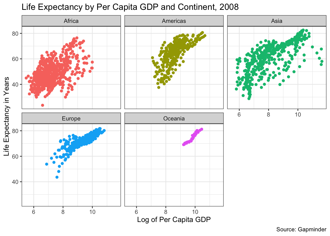
Finally, to ease the comparison of the two views we will add color as we did in the first graph. (Note the last line— theme(legend.position = "none") —eliminated the legend, which is unneeded here.)

ggplot(data = gapminder) + geom_point(mapping = aes(x= log(gdpPercap), y = lifeExp, color = continent)) +
  theme_bw() +
  ggtitle("Life Expectancy by Per Capita GDP and Continent, 2008") +
  labs(x = "Log of Per Capita GDP", y = "Life Expectancy in Years", caption = "Source: Gapminder") +
  facet_wrap(~ continent) +
  theme(legend.position = "none")