8.1 ANOVA

For ANOVA we will build on the states data example that examines high school graduation rates by region. [To review the two-variable analysis, look here.][Section 7.1.2]

To use ANOVA for a third variable, it must be a categorical variable. We will begin by managing our data to create a categorical variable from a quantitative variable. We will use state population, and divide it into three equally sized categories using the split_by command in the sjmisc package inside a mutate command. I added value labels to make for easier interpretation.

stateHSGradRate <-stateHSGradRate %>%
  mutate(popTotalCat = split_var(poptotal, n = 3))
stateHSGradRate$popTotalCat <- factor(stateHSGradRate$popTotalCat,
                                      levels = c(1,2,3),
                                      labels = c("Low Population", "Middle Population", "High Population"))

Now we can run the new three-variable model and look at the updated table of means for each sub-group.

The basic form of this model is as follows. (Remember you can copy this text!)

by(dataset, dataset$3rdVariable, function(x)
   list(aov(dependentVariable ~ independentVariable, data = x),
       summary(aov(dependentVariable ~ independentVariable, data = x))))

ftable(by(dataset$dependentVariable,
          list(dataset$independentVariable,
          dataset$3rdVariable), mean, na.rm= TRUE))

The code for our specific model is here:

by(stateHSGradRate, stateHSGradRate$popTotalCat, function(x)
   list(aov(gradRate ~ region, data = x),
       summary(aov(gradRate ~ region, data = x))))

## stateHSGradRate$popTotalCat: Low Population
## [[1]]
## Call:
##    aov(formula = gradRate ~ region, data = x)
## 
## Terms:
##                   region Residuals
## Sum of Squares  134.5651  130.9643
## Deg. of Freedom        3        13
## 
## Residual standard error: 3.173984
## Estimated effects may be unbalanced
## 
## [[2]]
##             Df Sum Sq Mean Sq F value Pr(>F)  
## region       3  134.6   44.86   4.452 0.0232 *
## Residuals   13  131.0   10.07                 
## ---
## Signif. codes:  0 '***' 0.001 '**' 0.01 '*' 0.05 '.' 0.1 ' ' 1
## 
## ------------------------------------------------------------ 
## stateHSGradRate$popTotalCat: Middle Population
## [[1]]
## Call:
##    aov(formula = gradRate ~ region, data = x)
## 
## Terms:
##                    region Residuals
## Sum of Squares   65.58333 183.41667
## Deg. of Freedom         3        12
## 
## Residual standard error: 3.909568
## Estimated effects may be unbalanced
## 
## [[2]]
##             Df Sum Sq Mean Sq F value Pr(>F)
## region       3  65.58   21.86    1.43  0.282
## Residuals   12 183.42   15.29               
## 
## ------------------------------------------------------------ 
## stateHSGradRate$popTotalCat: High Population
## [[1]]
## Call:
##    aov(formula = gradRate ~ region, data = x)
## 
## Terms:
##                    region Residuals
## Sum of Squares   42.13235 157.75000
## Deg. of Freedom         3        13
## 
## Residual standard error: 3.483477
## Estimated effects may be unbalanced
## 
## [[2]]
##             Df Sum Sq Mean Sq F value Pr(>F)
## region       3  42.13   14.04   1.157  0.363
## Residuals   13 157.75   12.13

ftable(by(stateHSGradRate$gradRate,
          list(stateHSGradRate$region, stateHSGradRate$popTotalCat), mean, na.rm= TRUE))

##            Low Population Middle Population High Population
##                                                            
## South            88.50000          85.50000        87.00000
## West             81.42857          82.33333        83.00000
## Midwest          87.00000          88.25000        84.50000
## Northeast        86.25000          88.00000        86.75000

We can assess regional differences for each of the population categories, low, middle, and high. The p-values are:

• Low population: .023
• Medium population: .282
• High population: .363

Only the low population states (.023) have within region differences that are statistically significant with a p-value below .05. The medium (.282) and high population states (.363) are both above .05.

The table shows that the South and West have the biggest differences between low population states.

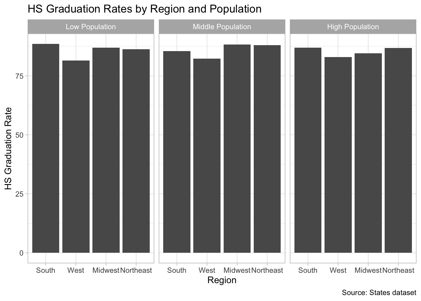
8.1.1 Representing this model in a faceted bar plot

To represent these three variables in a graph, we need to add one line to our two-variable graph, facet_wrap(), adding the third variable. Don’t forget the tilde ~.

ggplot(data= stateHSGradRate) + 
  stat_summary(mapping = aes(x = region, y = gradRate), fun= "mean", geom = "bar")  +
  ggtitle("HS Graduation Rates by Region and Population") +
  labs(x = "Region", y = "HS Graduation Rate", caption = "Source: States dataset") +
  theme_light() +
  facet_wrap(~ popTotalCat)