6.2 Scatterplot: Q -> Q
You create a scatterplot when you want to examine the relationship between two quantitative variables. To ease interpretation, you should place the independent (explanatory) variable along the x-axis, and the dependent (response) variable along the y-axis. We will look at examples using both States data and Gapminder data.
6.2.1 States Data
First, using States data, let’s examine the relationship between the percentage of a state’s population who are evangelical Christians (our independent variable) and the percentage of the state legislature who are women. The data is from 2011. There is only one year in this dataset, so no need to filter. If your data has multiple years, don’t forget to filter first! (You can look at the Gapminder example below.)
ggplot(data = my_usstate_data_2011_small, mapping = aes(x = evangelical_pop, y = pctfemaleleg)) +
  geom_point()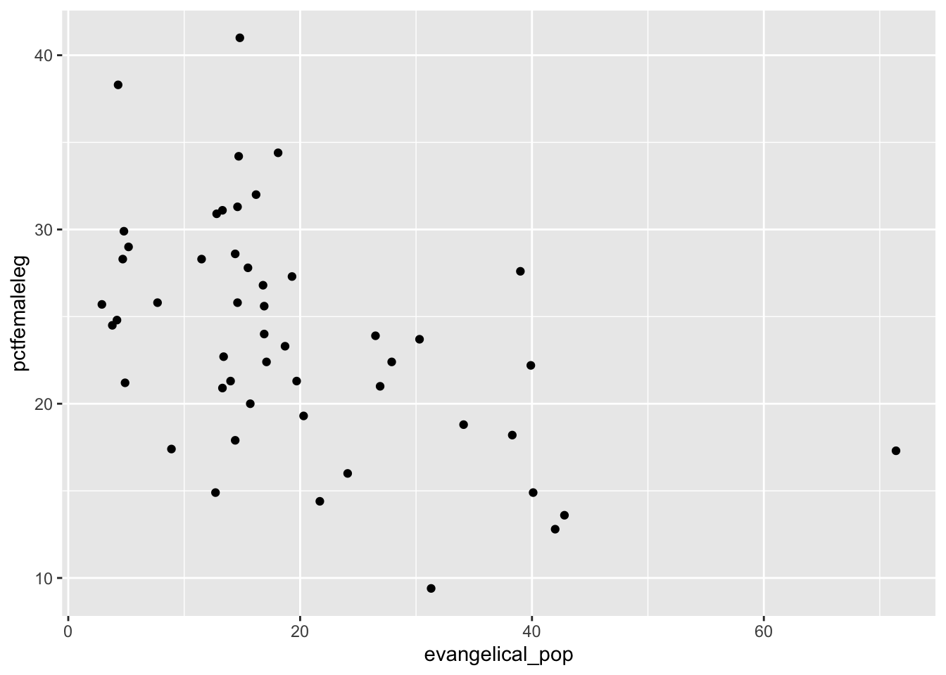
This basic plot works fine, but we will improve readability by making three changes. We will:
- Add axis labels and a title.
- Add a trend line to clarify the relationship between the two variables.
- Use a theme to make for a better appearance. We will use the built-in
theme_minimaltheme. https://ggplot2.tidyverse.org/reference/ggtheme.html If you are willing to install fonts onto your computer https://github.com/hrbrmstr/hrbrthemes 4. Want to add a third variable, like region? Look at the last Gapminder example for how to do this. (Add acolor =command in theaesstatement.)
ggplot(data = my_usstate_data_2011_small, mapping = aes(x = evangelical_pop, y = pctfemaleleg)) +
  geom_point() +
  ggtitle("Percentage of Women in State Legislatures \nby Percentage of Evangelical Christians, 2011")+
  labs(x = "Percentage of Evangelical Christians", y = "Percentage of Women in State Legislatures", caption = "Source: ICPPR State Data") +
  geom_smooth(method = lm, se = FALSE) +
  theme_minimal()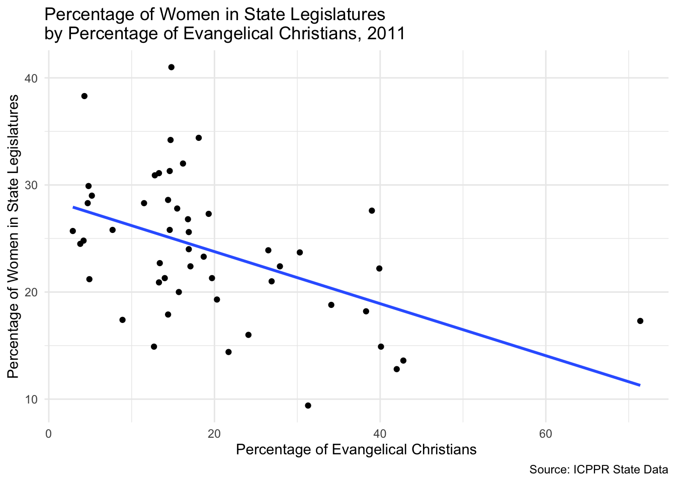
The trend line shows a significant negative relationship between a state’s evangelical population and the percentage of the state legislature that is women.
6.2.2 Gapminder Data
For this example, we will examine the relationship between a nation’s gross domestic product per capita and a nation’s life expectancy.
For this graph, we will need to filter out all but one year of data. We will use the filter command. We will combine this with creating the graph. Don’t forget to put the %>% and the + in the right places. As we did with the state data, we will also:
- Add axis labels and a title.
- Add a trend line to clarify the relationship between the two variables.
- Use a theme to make for a better appearance. For this, we will use the
theme_minimaltheme.
gapminder %>%
  filter(year == 2007) %>%
  ggplot(mapping = aes(x = gdpPercap, y = lifeExp)) +
  geom_point() +
  ggtitle("Life Expectancy by Per Capita Gross Domestic Product, 2007")+
  labs(x = "Per Capita Gross Domestic Product", y = "Life Expectancy (in years)", caption = "Source: Gapminder") +
  geom_smooth(method = lm, se = FALSE) +
  theme_classic()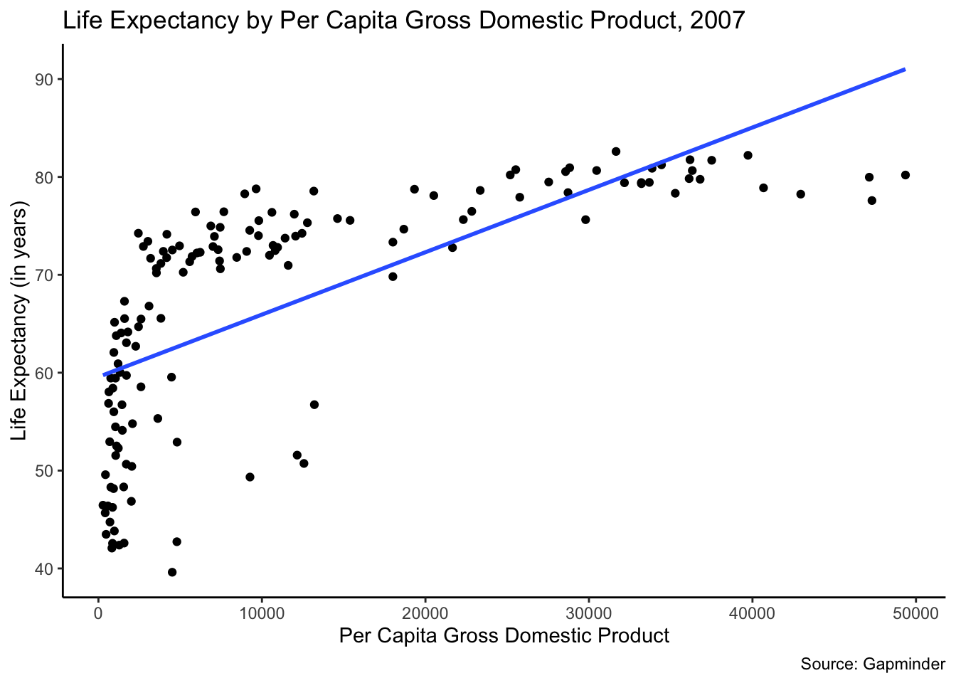
Note that this data has a curve up and to the right. There is a simple transformation we can make that will create an easier to interpret graph. We will use a log transformation of the per capita gross domestic product. (We will discuss why later.) We will wrap log() around our x-axis variable.
gapminder %>%
  filter(year == 2007) %>%
  ggplot(mapping = aes(x = log(gdpPercap), y = lifeExp)) +
  geom_point() +
  ggtitle("Life Expectancy by Per Capita Gross Domestic Product, 2007")+
  labs(x = "Log of Per Capita Gross Domestic Product", y = "Life Expectancy (in years)", caption = "Source: Gapminder") +
  geom_smooth(method = lm, se = FALSE) +
  theme_classic()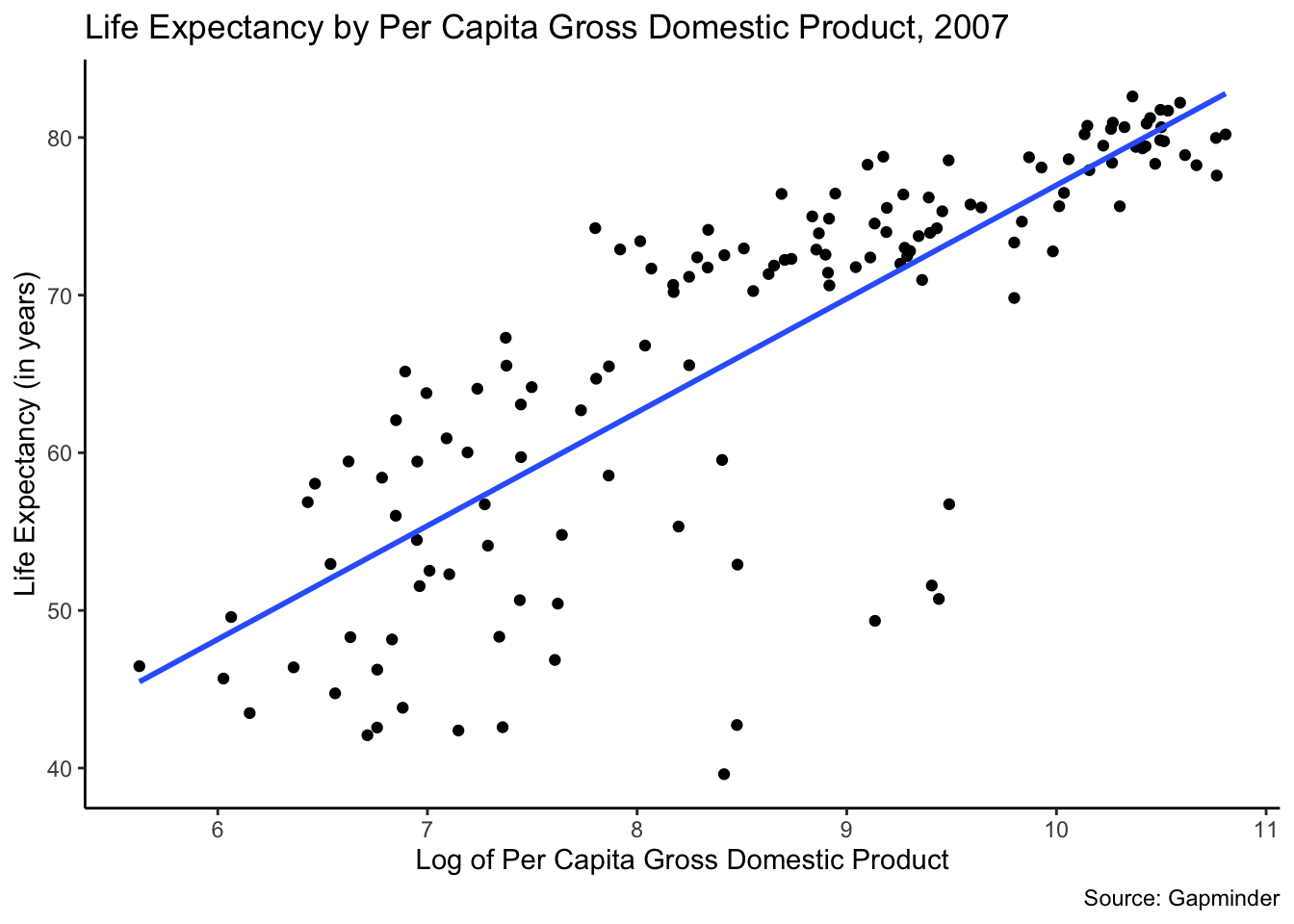
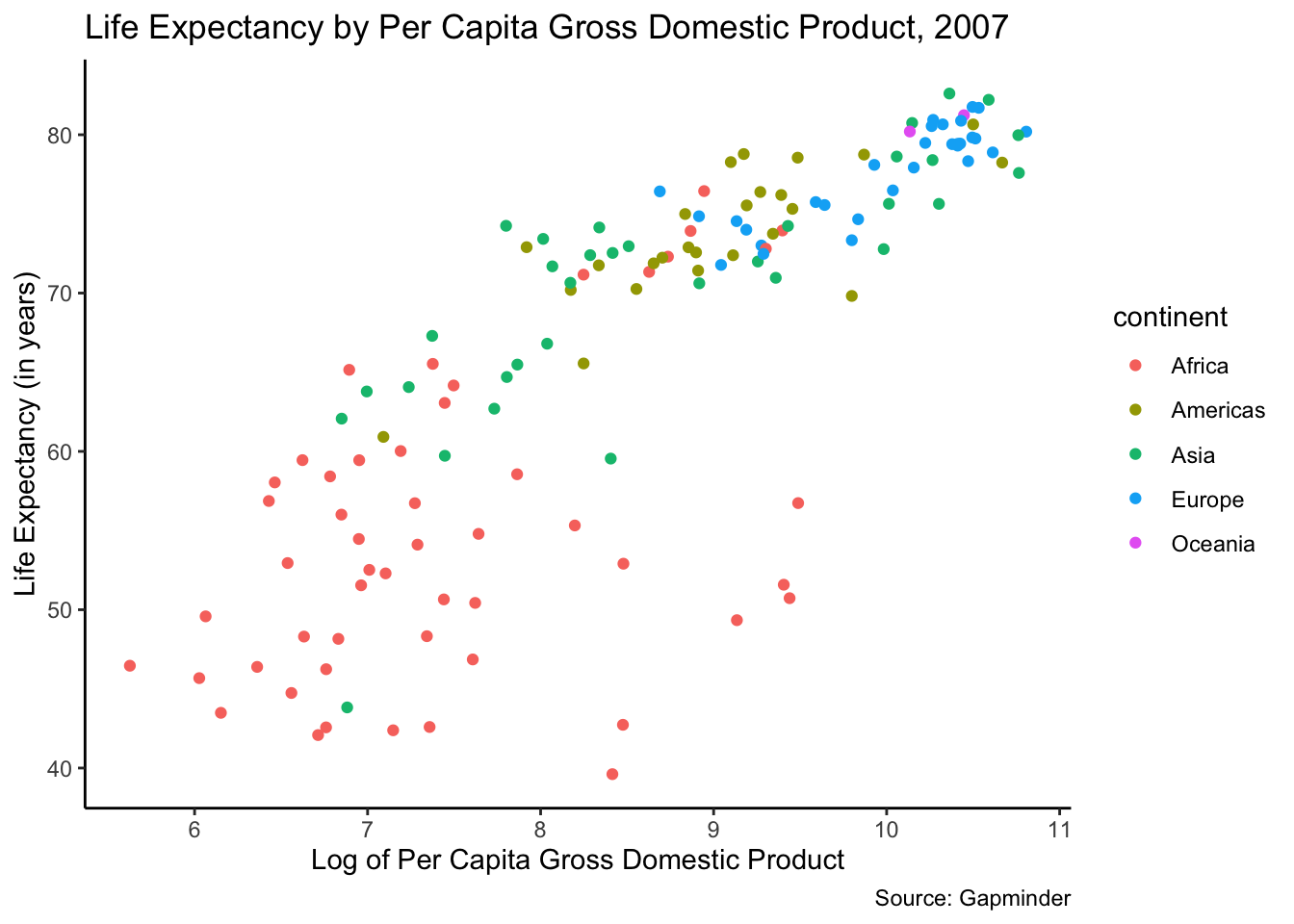
Finally, we can add a third variable to this graph. We will add continent here to give us a sense of how life expectancy differs, or not, between continents. To do this, add color = continent code in the aes statement. We will eliminate the trend line for simplicity. This third variable helps us understand the data better. Countries cluster within continents here.
gapminder %>%
  filter(year == 2007) %>%
  ggplot(mapping = aes(x = log(gdpPercap), y = lifeExp, color = continent)) +
  geom_point() +
  ggtitle("Life Expectancy by Per Capita Gross Domestic Product, 2007")+
  labs(x = "Log of Per Capita Gross Domestic Product", y = "Life Expectancy (in years)", caption = "Source: Gapminder") +
  theme_classic()