POLS 200 Tutorials
POLS 200 Tutorials for Passion Driven Statistics
Preface
1
Getting Ready to Work in RStudio
1.1
Installing RStudio
1.1.1
Downloading R on the Mac
1.1.2
Downloading R in Windows
1.1.3
Downloading RStudio
1.2
The RStudio layout
1.3
Where to store your files
1.4
Create an RStudio project
1.5
Open an RStudio project
1.6
Create an R script file
1.7
Running scripts
1.8
R packages
1.9
Installing R packages
1.9.1
The easy way:
1.9.2
The other way:
1.10
Loading packages
1.11
Setting your working directory
2
Taking a First Look at Your Data
2.1
Download your dataset
2.1.1
The World Values Survey
2.1.2
State Data from the IPPSR Site
2.1.3
Country Data from Gapminder
2.2
Load your dataset
2.2.1
Loading a World Values Study dataset
2.2.2
Loading a states dataset
2.2.3
Loading a Gapminder dataset
2.2.4
View your dataset
2.3
Displaying frequency distributions
2.4
Save your dataset
2.5
Compile your assignment
2.6
File examples
2.6.1
WVS data
2.6.2
States data
2.6.3
Gapminder data
3
Data management
3.1
Subsetting your dataset
3.2
Filtering data
3.2.1
An application
3.3
Recoding a variable
3.3.1
Recode a continuous variable to a categorical variable
3.3.2
Recode a new categorical variable from an existing categorical variable
3.4
Changing data types
3.5
Adding new Gapminder variables
3.6
Creating new variables
4
Exploring Data Analysis: Univariate Graphs
4.1
Background on ggplot
4.2
The Bar Graph: a graph for categorical variables
4.3
The Histogram: a graph for quantitative variables
4.4
A simple box plot: a graph for quantitative variables
5
Exploring Data Analysis: Univariate Statistics
5.1
Viewing univariate statistics
5.1.1
Skim
in
SkimR
5.1.2
descr
in
sjmisc
5.1.3
Summary
in Base R
5.1.4
Create a Codebook Using the Summarytools package
5.1.5
Single variables
6
Exploriatory Data Analysis: Two or more variables
6.1
Bar Graphs: C -> C, Q -> C, C -> Q
6.1.1
If your categorical dependent (response) variable has two categories
6.1.2
If your categorical dependent (response) variable has more than two categories
6.1.3
Recoding your categorical independent (explanatory) variable so that it has fewer categories
6.1.4
Creating a bar chart with a quantitative dependent (response) variable
6.2
Scatterplot: Q -> Q
6.2.1
States Data
6.2.2
Gapminder Data
6.3
The Two Variable Graph Flow Chart
7
Hypothesis Testing
7.1
Analysis of Variance: C -> Q
7.1.1
Example 1: Do OECD countries spend more money on education than non-OECD countries? (Gapminder)
7.1.2
Example 2: Do high school graduation rates vary by region? (States)
7.1.3
Example 3: Do Ethiopians vary by education level in how they evaluate whether “the army takes over when the government is incompetent” is “essential to democracy”? (WVS)
7.2
Chi-Square: C -> C, Q -> C
7.2.1
Example 1: Does Ethiopian’s assessment of respect for human rights vary by education? (WVS)
7.2.2
Example 2: Does Ethiopian’s national pride vary by education? (WVS)
7.3
Correlation: Q -> Q
7.3.1
Example 1: State population and the Gini Index
7.3.2
Example 2: GDP and life expectancy
7.3.3
Example 3: Does Ethiopian’s national pride vary by education? (WVS)
8
Moderation
8.1
ANOVA
8.1.1
Representing this model in a faceted bar plot
8.2
Chi-Square
8.2.1
Representing this model in a faceted bar plot
8.3
Correlation
8.3.1
Representing this model in a scatterplot
9
Regression Analysis
9.1
Linear Regression
9.1.1
Simple Linear Regression
9.1.2
Multiple Linear Regression
9.2
Logistic Regression
9.2.1
Simple Logistic Regression
9.2.2
Multiple Logistic Regression
Published with bookdown
POLS 200 Tutorials
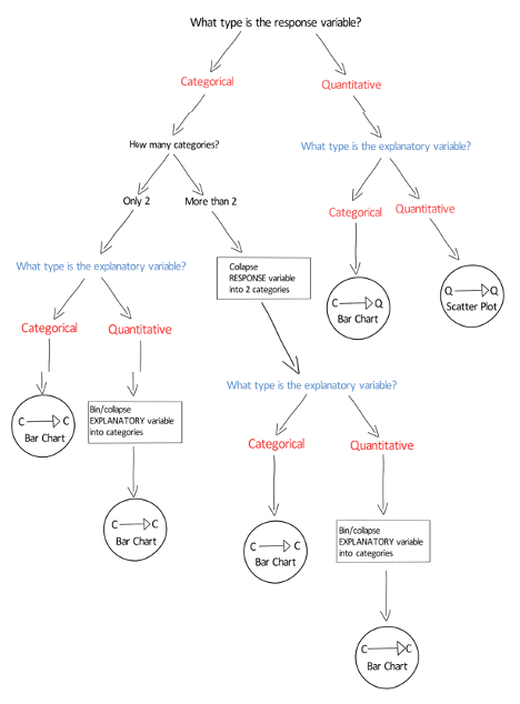
6.3
The Two Variable Graph Flow Chart