9.2 Logistic Regression
Logistic regression allows us to use a model very similar to regression. The model results look similar, although interpreting them is different. With logistic regression, we are developing models that show the probability that the dependent variable changes from one value to the other. We won’t use graphs here. We will use odds-ratios to interpret variables. There is no equivalent to R2 for logistic regression.
For more information on logistic regression go to the Introduction to Modern Statistics textbook.
9.2.1 Simple Logistic Regression
Running a logistic regression model in R is very similar to running linear regression. We will use the glm command instead of the lm command, and we need to add family = binomial at the end of the glm command. In addition to the summary command, we will also use exp and confint.
nameOfObject <- glm(dependentVariable ~ independentVariable1, data = dataset, family = "binomial")
summary(nameOfObject)
exp(nameOfObject$coefficients)
exp(confint(nameOfObject))
Example 1.
For a first example, we will use data from the National Election Study, a survey that is done in national election years of the US electorate. We will ask the question, does gender have an impact on who views Barak Obama positively in 2008? We will use a feeling thermometer question used in the NES. It asks people to rate a person or group from 0 (views very disfavorably) to 100 (views very favorably). The variable was recoded to create 2 groups, unfavorable is coded as 0 and favorable is coded as 1. The independent variable is gender.
We don’t create graphs to depict this model, we’ll go straight to the model.
obama_gender_glm <- glm(obamaThermSplit ~ gender, data = nesSmall, family = "binomial", weights = nes$wt)
summary(obama_gender_glm)
##
## Call:
## glm(formula = obamaThermSplit ~ gender, family = "binomial",
## data = nesSmall, weights = nes$wt)
##
## Deviance Residuals:
## Min 1Q Median 3Q Max
## -3.0225 -0.9712 0.5243 0.9453 2.5256
##
## Coefficients:
## Estimate Std. Error z value Pr(>|z|)
## (Intercept) 0.09122 0.03885 2.348 0.0189 *
## genderFemale 0.31112 0.05463 5.695 1.23e-08 ***
## ---
## Signif. codes: 0 '***' 0.001 '**' 0.01 '*' 0.05 '.' 0.1 ' ' 1
##
## (Dispersion parameter for binomial family taken to be 1)
##
## Null deviance: 7511.2 on 5494 degrees of freedom
## Residual deviance: 7478.6 on 5493 degrees of freedom
## (421 observations deleted due to missingness)
## AIC: 7124.2
##
## Number of Fisher Scoring iterations: 4## (Intercept) genderFemale
## 1.095514 1.364956## 2.5 % 97.5 %
## (Intercept) 1.015220 1.182264
## genderFemale 1.226446 1.519322In interpreting our model, we can want to look at three things:
- the test of statistical significance, the z-test,
- the coefficient
- confidence intervals of the coefficient
- note there is no equivalent of R2 for logistic regression.
These models use odds ratios rather than direct numerical parameters.
The test of statistical significance. We want to look at the Pr(>|z|) column to assess the z-score. If Pr(>|z|) is less than .05 we can state that the relationship is statistically significant. We reject the null hypothesis. For this model, the probability is 1.23e-08, much lower than .05.
The coefficient. We can look at the coefficient of both the dependent variable and the independent variable. In this instance they are:
- Opinion of Barak Obama: 1.10. A person surveyed was 1.1 times more likely to have a positive opinion of Obama.
- Gender: 1.36. Women are 1.36 times more likely to have a positive opinion of Obama than men.
Confidence intervals of the coefficient. For gender, we can have 95% confidence that additional samples would have an odds ratio for gender between 1.23 and 1.52.
Example 2.
We will use the World Value Survey from Ethiopia for our second example. We will ask the question, does education level impact Ethiopian’s views of human rights in their country? To run the analysis, I created a new human rights variable, Q253_recode, dividing responses into less respect for human rights and more respect for human rights. Education Q275R is divided into three groups, lower, middle, and higher.
We don’t create graphs to depict this model first. We’ll go straight to the model.
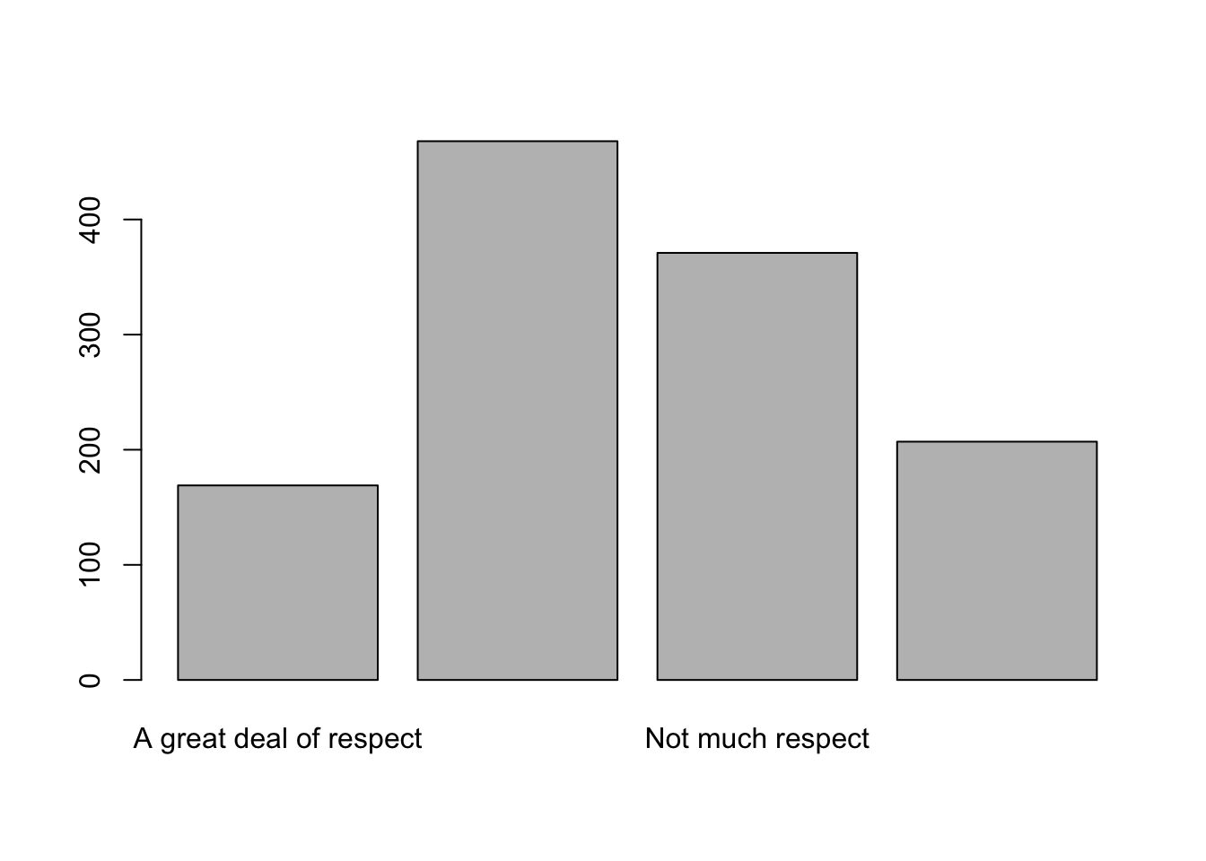
## Respect for individual human rights nowadays
##                         Frequency Percent Valid Percent
## A great deal of respect       169   13.74         13.91
## Fairly much  respect          468   38.05         38.52
## Not much respect              371   30.16         30.53
## No respect at all             207   16.83         17.04
## NA's                           15    1.22
## Total 1230 100.00 100.00ethiopia_small$Q253_recode <- fct_collapse(ethiopia_small$Q253,
"Less Respect" = c("Not much respect", "No respect at all"),
"More Respect" = c("A great deal of respect", "Fairly much respect"))
freq(ethiopia_small$Q253_recode)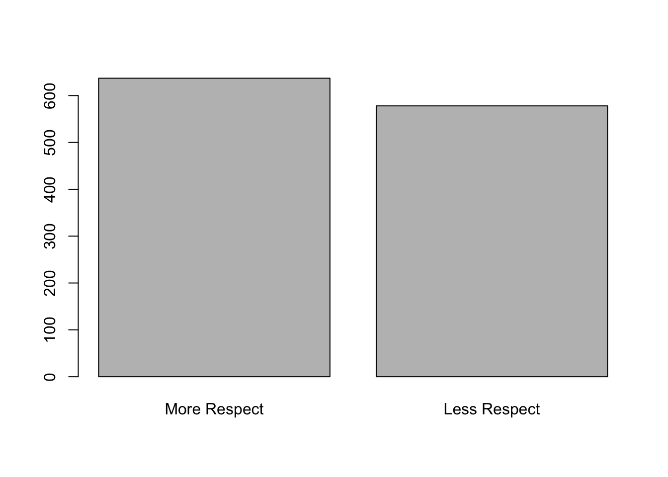
## Respect for individual human rights nowadays
##              Frequency Percent Valid Percent
## More Respect       637   51.79         52.43
## Less Respect       578   46.99         47.57
## NA's                15    1.22
## Total             1230  100.00        100.00
## run model
ethiopia_hr_glm <- glm(Q253_recode ~ Q275R, data = ethiopia_small, family = "binomial")
summary(ethiopia_hr_glm)##
## Call:
## glm(formula = Q253_recode ~ Q275R, family = "binomial", data = ethiopia_small)
##
## Deviance Residuals:
## Min 1Q Median 3Q Max
## -1.267 -1.096 -1.096 1.261 1.261
##
## Coefficients:
## Estimate Std. Error z value Pr(>|z|)
## (Intercept) -0.19349 0.07158 -2.703 0.00687 **
## Q275RMiddle 0.40171 0.14799 2.714 0.00664 **
## Q275RHigher 0.12680 0.16544 0.766 0.44340
## ---
## Signif. codes: 0 '***' 0.001 '**' 0.01 '*' 0.05 '.' 0.1 ' ' 1
##
## (Dispersion parameter for binomial family taken to be 1)
##
## Null deviance: 1673.3 on 1208 degrees of freedom
## Residual deviance: 1665.9 on 1206 degrees of freedom
## (21 observations deleted due to missingness)
## AIC: 1671.9
##
## Number of Fisher Scoring iterations: 3In interpreting our model, we can want to look at three things:
- the test of statistical significance, the z-test,
- the coefficient
- confidence intervals of the coefficient
- note there is no equivalent of R2 for logistic regression.
These models use odds ratios rather than direct numerical parameters.
The test of statistical significance. We want to look at the Pr(>|z|) column to assess the z-score. If Pr(>|z|) is less than .05 we can state that the relationship for those with medium education is statistically significant. We reject the null hypothesis. For this model, the probability for medium education is 00687, much lower than .05 and .44 for higher education, above .05. We cannot reject the null hypothesis for those with higher education.
The coefficient. We can look at the coefficient of both the dependent variable and the independent variable. They are:
- Ethiopia supports human rights: .82. A person surveyed was .82 times more likely to have a positive opinion of Obama.
- Middle Education: 1.49. Ethiopians with middle levels of education are 1.49 times more likely to believe that human rights are respected in Ethiopia.
- Higher Education: 1.13. Ethiopians with higher levels of education are 1.13 times more likely to believe that human rights are respected in Ethiopia.
Confidence intervals of the coefficient. For middle levels of education, we can have 95% confidence that additional samples would have an odds ratio for gender between 1.19 and 2.00.
9.2.2 Multiple Logistic Regression
Linear regression is also very flexible and allows for several, even many, independent (explanatory) variables. The general model only changes in that we add more variables with a + sign between each independent (explanatory) variable.
nameOfObject <- glm(dependentVariable ~ independentVariable1 + independentVariable2, data = dataset, family = "binomial")
summary(nameOfObject)
exp(nameOfObject$coefficients)
exp(confint(nameOfObject))
Example 1. For this model, we will add political party (pid_3) to our original model. Democrats are coded as 0, independents are coded as 1, and Republicans are coded as 2.
obama_gender_party_glm <- glm(obamaThermSplit ~ gender + pid_3, data = nesSmall, family = "binomial", weights = nes$wt)
summary(obama_gender_party_glm)
##
## Call:
## glm(formula = obamaThermSplit ~ gender + pid_3, family = "binomial",
## data = nesSmall, weights = nes$wt)
##
## Deviance Residuals:
## Min 1Q Median 3Q Max
## -4.7561 -0.5939 0.2478 0.5804 4.3005
##
## Coefficients:
## Estimate Std. Error z value Pr(>|z|)
## (Intercept) 2.21597 0.08886 24.939 < 2e-16 ***
## genderFemale 0.25063 0.06878 3.644 0.000268 ***
## pid_3Ind -2.18955 0.09263 -23.637 < 2e-16 ***
## pid_3Rep -4.09287 0.10918 -37.489 < 2e-16 ***
## ---
## Signif. codes: 0 '***' 0.001 '**' 0.01 '*' 0.05 '.' 0.1 ' ' 1
##
## (Dispersion parameter for binomial family taken to be 1)
##
## Null deviance: 7488 on 5473 degrees of freedom
## Residual deviance: 5213 on 5470 degrees of freedom
## (442 observations deleted due to missingness)
## AIC: 4957
##
## Number of Fisher Scoring iterations: 4## (Intercept) genderFemale pid_3Ind pid_3Rep
## 9.17026184 1.28483161 0.11196750 0.01669127## 2.5 % 97.5 %
## (Intercept) 7.72828624 10.95070537
## genderFemale 1.12289322 1.47043576
## pid_3Ind 0.09311896 0.13391531
## pid_3Rep 0.01343450 0.02061339In interpreting our model, we can want to look at three things:
- the test of statistical significance, the z-test,
- the coefficient
- confidence intervals of the coefficient
- note there is no equivalent of R2 for logistic regression.
These models use odds ratios rather than direct numerical parameters.
The test of statistical significance. We want to look at the Pr(>|z|) column to assess the z-score. If Pr(>|z|) is less than .05 we can state that the relationship for those with medium education is statistically significant. We reject the null hypothesis. For this model, each of the variables is statistically significant.
The coefficient. We can look at the coefficient of both the dependent variable and the independent variable. In this instance they are:
- Opinion of Barak Obama: 9.17.
- Gender: 1.28.
- Independent: .117.
- Republican: .02.
Confidence intervals of the coefficient.
Example 2.
For this model, we will add gender (Q260) to our original model.
ethiopia_multi_glm <- glm(Q253_recode ~ Q275R + Q260, data = ethiopia_small,  family = "binomial")
summary(ethiopia_multi_glm)
##
## Call:
## glm(formula = Q253_recode ~ Q275R + Q260, family = "binomial",
## data = ethiopia_small)
##
## Deviance Residuals:
## Min 1Q Median 3Q Max
## -1.282 -1.113 -1.081 1.243 1.277
##
## Coefficients:
## Estimate Std. Error z value Pr(>|z|)
## (Intercept) -0.15370 0.09364 -1.641 0.10073
## Q275RMiddle 0.39656 0.14821 2.676 0.00746 **
## Q275RHigher 0.11671 0.16617 0.702 0.48248
## Q260Female -0.07643 0.11614 -0.658 0.51048
## ---
## Signif. codes: 0 '***' 0.001 '**' 0.01 '*' 0.05 '.' 0.1 ' ' 1
##
## (Dispersion parameter for binomial family taken to be 1)
##
## Null deviance: 1673.3 on 1208 degrees of freedom
## Residual deviance: 1665.5 on 1205 degrees of freedom
## (21 observations deleted due to missingness)
## AIC: 1673.5
##
## Number of Fisher Scoring iterations: 3## (Intercept) Q275RMiddle Q275RHigher Q260Female
## 0.8575276 1.4867032 1.1237906 0.9264197## 2.5 % 97.5 %
## (Intercept) 0.7134056 1.030035
## Q275RMiddle 1.1126476 1.990152
## Q275RHigher 0.8108039 1.556495
## Q260Female 0.7377325 1.163237The test of statistical significance. We want to look at the Pr(>|z|) column to assess the z-score. If Pr(>|z|) is less than .05 we can state that the relationship for those with medium education is statistically significant. We reject the null hypothesis. For this model, only the middle level of education is statistically significant.
- Ethiopia supports human rights: .85.
- Middle Education: 1.49.
- Higher Education: 1.12.
- Female: .92.