7.1 Analysis of Variance: C -> Q
Analysis of variance (ANOVA) is the appropriate statistical test when your hypothesis includes an independent (explanatory) variable that is categorical and a dependent (response) variable that is quantitative. The PDS Video explains the basic assumptions of using ANOVA. For more information on ANOVA go to the OpenStax statistics textbook.
For each model, your procedure is as follows:
- Manage your data as needed.
- Specify your model and look at the summary.
- Look at a box plot of your data.
- Examine the means of your data.
- If needed, run the post-hoc test to look at which categories are statistically significant.
To run ANOVA and related procedures, you will need to load the Tidyverse and sjmisc packages.
In the rest of this section, we will walk through three examples.

7.1.1 Example 1: Do OECD countries spend more money on education than non-OECD countries? (Gapminder)
With this example, we will test the following hypothesis: OECD countries spend more money on education than non-OECD countries.
We are taking this data from the Gapminder dataset.
7.1.1.1 Managing the data
The variable studentSpendingPerCapita does not need any management, but I don’t have a variable that is coded OECD country or not an OECD country. There is a variable, g77_and_oecd_countries, with the data I need, however. I will recode it so that we get the data we need by recoding the “g77” and “other” categories as “non-OECD”. Run frequency distributions before and after to make sure I recoded correctly. We have 28 OECD countries in each variable and, the total of G77 and other countries add up to the total recoded as non-OECD. We can now move forward.
## Frequencies
## my_gapminder_data_2003$g77_and_oecd_countries
## Type: Character
##
##                Freq   % Valid   % Valid Cum.   % Total   % Total Cum.
## ------------ ------ --------- -------------- --------- --------------
##          g77    102     67.55          67.55     62.58          62.58
##         oecd     28     18.54          86.09     17.18          79.75
##       others     21     13.91         100.00     12.88          92.64
##         <NA>     12                               7.36         100.00
## Total 163 100.00 100.00 100.00 100.007.1.1.2 Specify the model and review the summary
We can now run our model. We do this using the aov command in base R. (No new packages are needed.)
The basic form is as follows:
nameOfObject <- aov(dependentVariable ~ independentVariable, data = DatasetName)Here is the first example.
- object: student_spend_oecd_aov
- dependent variable: studentSpendingPerCapita
- independent variable: g77_and_oecd_countries_r
- dataset: myGapminderData2003
We run the model, create the object, and then run the summary command to look at the results.
student_spend_oecd_aov <- aov(studentSpendingPerCapita ~ g77_and_oecd_countries_recode, data = my_gapminder_data_2003)
summary(student_spend_oecd_aov)
## Df Sum Sq Mean Sq F value Pr(>F)
## g77_and_oecd_countries_recode 1 0.02878 0.028784 11.68 0.0012 **
## Residuals 55 0.13555 0.002465
## ---
## Signif. codes: 0 '***' 0.001 '**' 0.01 '*' 0.05 '.' 0.1 ' ' 1
## 106 observations deleted due to missingnessAs discussed in the video, the key number is the measure of statistical significance “Pr(>F)”. If that number is smaller than .05 the relationship between the two variables is statistically significant. The F-Test is .0012, smaller than .05. We can reject the null hypothesis and accept that our hypothesis–OECD countries spend more money on education than non-OECD countries–is confirmed.
7.1.1.3 Create and review the box plot
The box plot allows us to visualize this relationship.
Watch a video explaining how to read a box plot. Here is a statistics text on the box plot.
my_gapminder_data_2003 %>%
  filter(!is.na(g77_and_oecd_countries_recode)) %>%
  ggplot() + geom_boxplot(mapping = aes(x = g77_and_oecd_countries_recode, y = studentSpendingPerCapita)) +
  theme_minimal()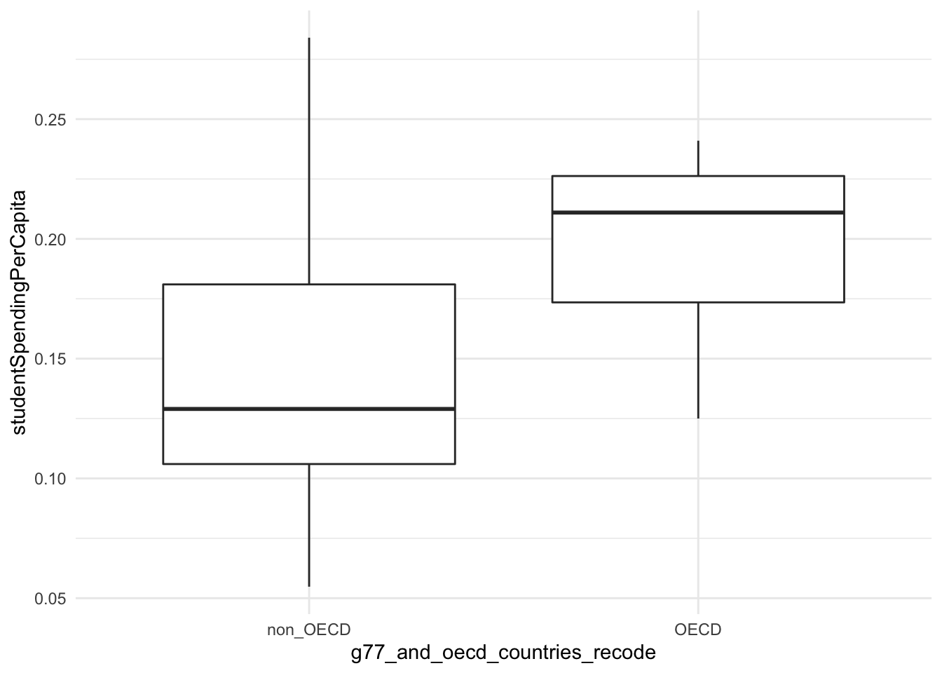
Looking at this box plot, we can see that spending is very different between OECD and non-OECD countries. The medians are notably different (.13 vs. .21), noted by the bar in the middle of the box and the interquartile means for non-OECD countries are much lower(.11-.18) as compared to OECD countries (.17-.23)
7.1.1.4 Produce the means and review
The differences we see in the ANOVA, and the box plot are also reflected in the means of the two groups with the OECD countries being higher.
my_gapminder_data_2003 %>%
  filter(!is.na(g77_and_oecd_countries_recode)) %>%
  group_by(g77_and_oecd_countries_recode) %>%
  summarize(meanStudentSpending = mean(studentSpendingPerCapita, na.rm=TRUE))
## # A tibble: 2 x 2
## g77_and_oecd_countries_recode meanStudentSpending
## * <fct> <dbl>
## 1 non_OECD 0.144
## 2 OECD 0.1947.1.1.5 Do Post-Hoc Testing
Because there are only two categories in the independent variable, we do not need to do post-hoc testing for this model.
7.1.2 Example 2: Do high school graduation rates vary by region? (States)
With this example, we will test the following hypotheses.
- There is a significant difference between high school graduation rates in the four US regions.
- The Northeast has significantly higher high school graduation rates than the other three regions (the Midwest, West, and the South).
We are taking this data from the States dataset. The data for the second example is as follows:
- object: state_hs_grad_aov
- dependent variable: gradRate
- independent variable: region
- dataset: state_hs_grad_rate
7.1.2.1 Managing the data
Originally the region variable was coded 1-4. Earlier I added labels to make interpretation easier. Below is the code I used.
state_hs_grad_rate$region <- factor(state_hs_grad_rate$region,
                    levels = c(1,2,3,4),
                    labels = c("South", "West", "Midwest", "Northeast"))
Here is the frequency distribution of the regions.
##
## x <categorical>
## # total N=50  valid N=50  mean=2.28  sd=1.11
##
## Value     |  N | Raw % | Valid % | Cum. %
## -----------------------------------------
## South     | 16 |    32 |      32 |  32.00
## West      | 13 |    26 |      26 |  58.00
## Midwest   | 12 |    24 |      24 |  82.00
## Northeast |  9 |    18 |      18 | 100.00
## <NA>      |  0 |     0 |    <NA> |   <NA>
7.1.2.2 Specify the model and review the summary
After running the model and the summary we see that the F-test shows a probability of .00193. It is lower than .05, so we can reject the null hypothesis of our first hypothesis. Regional high school graduation rates vary in a statistically significant way.
##             Df Sum Sq Mean Sq F value  Pr(>F)
## region       3  198.7   66.22   5.782 0.00193 **
## Residuals   46  526.9   11.45
## ---
## Signif. codes:  0 '***' 0.001 '**' 0.01 '*' 0.05 '.' 0.1 ' ' 1
7.1.2.3 Create and review the box plot
Based on the box plot, it is not surprising that the differences between the groups are statistically significant.
We can see that overall the West has lower high school graduation rates. The other three regions vary in how tightly cluster they are, the interquartile ranges vary, but the medians are very similar.
state_hs_grad_rate %>%
  ggplot() + geom_boxplot(mapping = aes(x = region, y = gradRate)) +
  theme_minimal()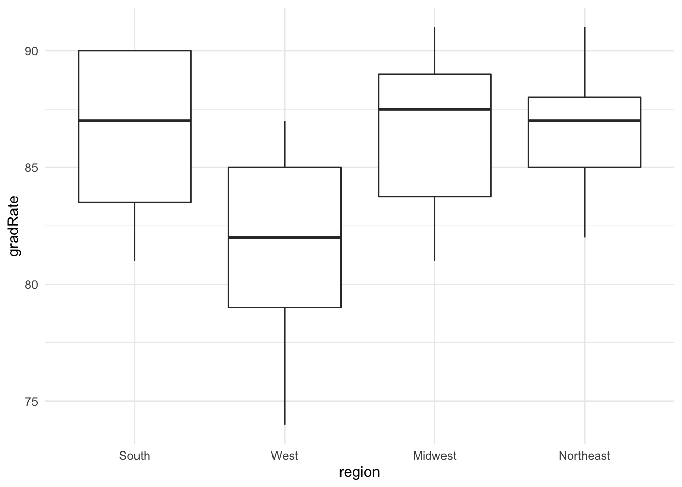
7.1.2.4 Produce the means and review
Based on the means below and the box plot above, it is questionable that my second hypothesis—that the Northeast has higher graduation rates than the other regions—will be confirmed. While it has the highest mean, 86.67, it isn’t much higher than the Midwest and the South. Similar to the box plot, the mean of the West is lower than the other three regions.
## # A tibble: 4 x 2
##   region    meanHSGradRate
## * <fct>              <dbl>
## 1 South               86.4
## 2 West                82
## 3 Midwest             86.6
## 4 Northeast           86.7
7.1.2.5 Do Post-Hoc Testing
To test the second hypothesis and to understand where the significant differences are between regions, we will conduct a post-hoc test, the Tukey HSD (honestly significant difference) test. This test compares all of the differences between pairs as discussed in the video.
##   Tukey multiple comparisons of means
##     95% family-wise confidence level
##
## Fit: aov(formula = gradRate ~ region, data = state_hs_grad_rate)
##
## $region
##                          diff        lwr       upr     p adj
## West-South        -4.43750000 -7.8058073 -1.069193 0.0053918
## Midwest-South      0.14583333 -3.2990362  3.590703 0.9994782
## Northeast-South    0.22916667 -3.5294941  3.987827 0.9984498
## Midwest-West       4.58333333  0.9721289  8.194538 0.0077613
## Northeast-West     4.66666667  0.7549915  8.578342 0.0135623
## Northeast-Midwest  0.08333333 -3.8944593  4.061126 0.9999365
To interpret this table, look at the “p adj” in the table. If the adjusted p-value is lower than .05 we can say the difference between the pair is statistically significant. Three pairs meet this criterion.
- West-South
- Midwest-West
- Northeast-West
So we can’t confirm that the Northeast states have higher graduation rates than the other regions. We can, though, confirm that the West has statistically significantly lower high school graduation rates than the other three regions.
7.1.3 Example 3: Do Ethiopians vary by education level in how they evaluate whether “the army takes over when the government is incompetent” is “essential to democracy”? (WVS)
With this example, we will test the following hypothesis.
- There is a significant difference between high school graduation rates in the four US regions.
- Ethiopians with higher levels of education are significantly more likely to think that the army takes over when the government is incompetent is essential to democracy than people with lower levels of education.
These are both categorical variables, but because the dependent variable has ten categories, we can treat it as quantitative.
We are taking this data from the WVS dataset. The data for the second example is as follows:
- object: ethiopia_mil_dem_aov
- dependent variable: Q246New
- independent variable: Q275RNew
- dataset: ethiopia_small
7.1.3.1 Specify the model and review the summary
We need to make a small change here. ANOVA only works with numeric data. We will use the as.numeric command with Q246.
## Frequencies
## ethiopia_small$Q246
## Label: Democracy: Civil rights protect people’s liberty against oppression
## Type: Factor
##
##                                                      Freq   % Valid   % Valid Cum.   % Total   % Total Cum.
## -------------------------------------------------- ------ --------- -------------- --------- --------------
##       Not an essential characteristic of democracy     95      8.36           8.36      7.72           7.72
##                                                  2     17      1.50           9.85      1.38           9.11
##                                                  3     11      0.97          10.82      0.89          10.00
##                                                  4     11      0.97          11.79      0.89          10.89
##                                                  5     29      2.55          14.34      2.36          13.25
##                                                  6     42      3.69          18.03      3.41          16.67
##                                                  7     52      4.57          22.60      4.23          20.89
##                                                  8     94      8.27          30.87      7.64          28.54
##                                                  9    158     13.90          44.77     12.85          41.38
##           An essential characteristic of democracy    628     55.23         100.00     51.06          92.44
##                                               <NA>     93                               7.56         100.00
## Total 1230 100.00 100.00 100.00 100.00## Frequencies
## ethiopia_small$Q275R
## Label: Highest educational level: Respondent (recoded into 3 groups)
## Type: Factor
##
## Freq % Valid % Valid Cum. % Total % Total Cum.
## ------------ ------ --------- -------------- --------- --------------
## Lower 803 65.60 65.60 65.28 65.28
## Middle 241 19.69 85.29 19.59 84.88
## Higher 180 14.71 100.00 14.63 99.51
## <NA> 6 0.49 100.00
## Total 1230 100.00 100.00 100.00 100.00## Df Sum Sq Mean Sq F value Pr(>F)
## Q275R 2 3 1.572 0.202 0.817
## Residuals 1129 8762 7.761
## 98 observations deleted due to missingnessAfter running the model, we can see no significant difference between evaluations of the importance of the “army takes over when government is incompetent” to democracy. The probability of the F-test is .817, much higher than the .05 significance level. We cannot reject the null hypothesis.
7.1.3.2 Create and review the box plot
We see that the box plot shows that the distributions of the data are very similar.
ethiopia_small %>%
  filter(!is.na(Q275R)) %>%
  ggplot() + geom_boxplot(mapping = aes(x = Q275R, y = Q246)) +
  theme_minimal()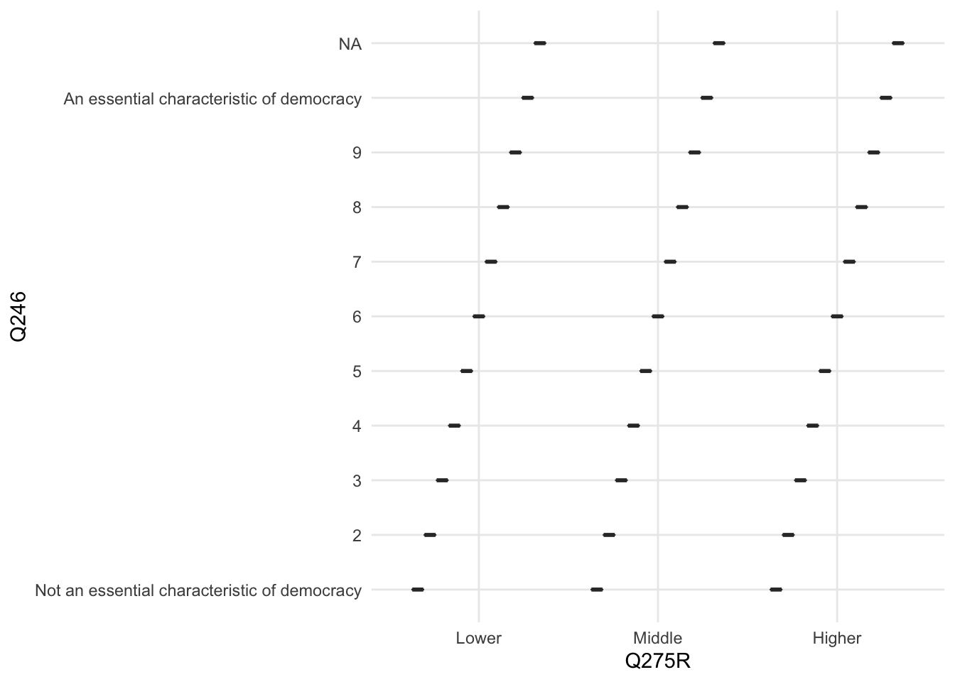
7.1.3.3 Produce the means and review
The means are too quite similar. Both the means and the box plot reinforce what we learned in the ANOVA.
ethiopia_small %>%
  filter(!is.na(Q275R)) %>%
  group_by(Q275R) %>%
  summarize(meanQ246 = mean(Q246, na.rm=TRUE))
## # A tibble: 3 x 2
## Q275R meanQ246
## * <fct> <dbl>
## 1 Lower NA
## 2 Middle NA
## 3 Higher NA7.1.3.4 Do Post-Hoc Testing## Manage data state regions have labels using
The post-hoc test shows no statistically significant relationships between the pairs, as we would expect based on the ANOVA results.
##   Tukey multiple comparisons of means
##     95% family-wise confidence level
##
## Fit: aov(formula = as.numeric(Q246) ~ Q275R, data = ethiopia_small)
##
## $Q275R
##                      diff        lwr       upr     p adj
## Middle-Lower  0.007497447 -0.4846909 0.4996858 0.9992957
## Higher-Lower  0.148379770 -0.4059769 0.7027364 0.8046765
## Higher-Middle 0.140882324 -0.5163610 0.7981257 0.8698589