7.3 Correlation: Q -> Q
In comparison to ANOVA and chi-square tests, looking at Pearson correlation is simple. You can (watch the PDS video here)[https://www.youtube.com/watch?v=lf4HfHx2ASs&list=PL2fQHGEDK7YzW-06PZYcboa1IfcqTSil-&index=12]. And get more information in (the OpenStax statistics text here)[https://openstax.org/books/introductory-statistics/pages/12-4-testing-the-significance-of-the-correlation-coefficient].
For each test your procedure is as follows:
- Run the Pearson correlation test.
- Run a scatterplot to examine the shape of the data.
We will look at two examples with data from the States dataset and the Gapminder dataset.

7.3.1 Example 1: State population and the Gini Index
With this example we will test the following hypotheses:
- As a state population goes up, a state’s high school graduation rate will go up.
- As a state’s Gini Index goes up, a state’s high school graduation rate will go down.
We are taking this data from the States dataset.
7.3.1.1 Run the Pearson correlation tests
We are interested in two measures here, the Pearson’s correlation and the p-value test of statistical significance. Correlation varies from -1 to +1. With -1 and +1 being a perfect correlation and 0 indicating no correlation. For the p-value we need it to be less than .05 to have statistical significance, allowing us to reject the null hypothesis.
For our first test, the correlation is .01, very close to zero. It is positive so it moves in the direction we expected. The p-value however is .94, much higher than .05. We cannot reject the null hypothesis. There is not a statistically significant relationship.
For our second test, the correlation is -.014, very close to zero. It is negative so it moves in the direction we expected. The p-value however is .92, much higher than .05. We cannot reject the null hypothesis. There is not a statistically significant relationship.
##
##  Pearson's product-moment correlation
##
## data:  state_hs_grad_rate$gradRate and state_hs_grad_rate$poptotal
## t = 0.075289, df = 48, p-value = 0.9403
## alternative hypothesis: true correlation is not equal to 0
## 95 percent confidence interval:
##  -0.2682928  0.2883420
## sample estimates:
##        cor
## 0.01086642##
## Pearson's product-moment correlation
##
## data: state_hs_grad_rate$gradRate and state_hs_grad_rate$giniIndex
## t = -0.10066, df = 48, p-value = 0.9202
## alternative hypothesis: true correlation is not equal to 0
## 95 percent confidence interval:
## -0.2916957 0.2648913
## sample estimates:
## cor
## -0.014527547.3.1.2 Run the scatterplots
These tests are reinforced by the two scatterplots. Each has a flat trend line—the first positive (moving ever slow slightly up from left to right) and the other negative (moving ever slow slightly down from left to right)—indicating a weak relationship.
ggplot(data = state_hs_grad_rate, mapping = aes(x = poptotal, y = gradRate)) +
  geom_point() +
  ggtitle("State High School Graduation Rates by State Median Income, 2017")+
  labs(x = "State Median Income (in 1,000s of dollars)", y = "State HS Graduation Rates (in percent)", caption = "Source: Wikipedia") +
  geom_smooth(method = lm, se = FALSE) +
  theme_minimal()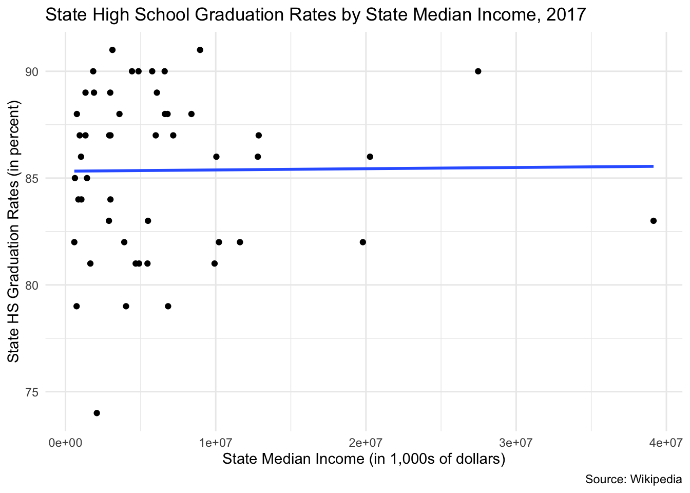
ggplot(data = state_hs_grad_rate, mapping = aes(x = giniIndex, y = gradRate)) +
  geom_point() +
  ggtitle("State High School Graduation Rates by State Gini Index, 2017")+
  labs(x = "State Gini Index", y = "State HS Graduation Rates (in percent)", caption = "Source: Wikipedia") +
  geom_smooth(method = lm, se = FALSE) +
  theme_minimal()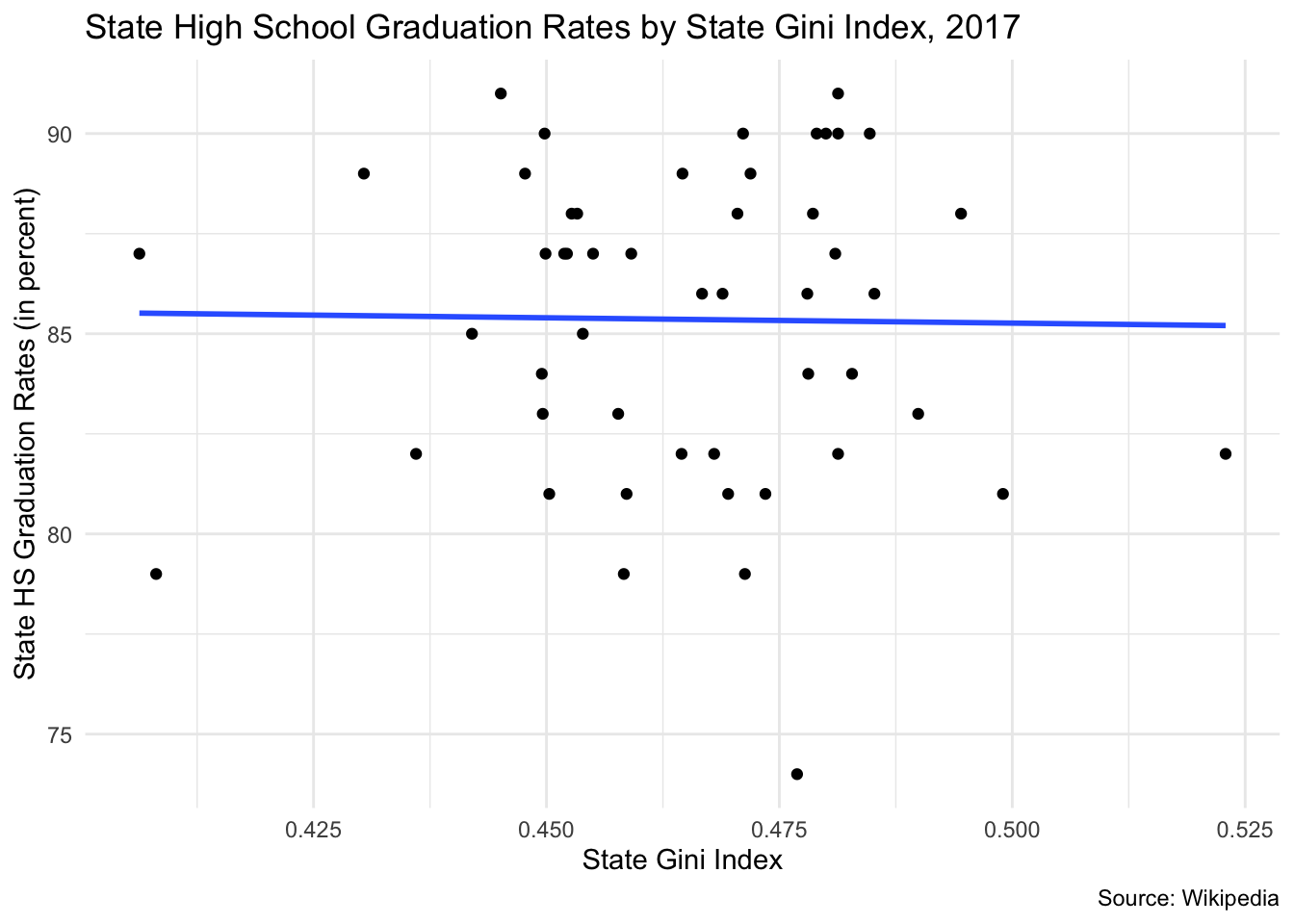
7.3.2 Example 2: GDP and life expectancy
With this example we will test the following hypothesis:
- As a nation’s GDP goes up, a nation’s life expectancy will go up.
- As a nation’s population goes up, a nation’s life expectancy will go down.
We are taking this data from the Gapminder dataset.
7.3.2.1 Run the Pearson correlation tests
We are interested in two measures here, the Pearson’s correlation and the p-value test of statistical significance. Correlation varies from -1 to +1. With -1 and +1 being a perfect correlation and 0 indicating no correlation. For the p-value we need it to be less than .05 to have statistical significance, allowing us to reject the null hypothesis.
For our first test, the correlation is .584, quite high. It is positive so it moves in the direction we expected. The p-value however is .0000, lower than .05. We can reject the null hypothesis. There is a statistically significant relationship.
For our second test, the correlation of .065, close to zero. It is positive so it moves in the direction we expected. Despite the modest correlation, the p-value however is .007, lower than .05. We can reject the null hypothesis. There is not a statistically significant relationship.
In thinking about the percentage of the variance that is explained, r2, our first test explains 33.6% of the variance. Our second test explains 0.4% of the variance.
##
##  Pearson's product-moment correlation
##
## data:  gapminder$lifeExp and gapminder$gdpPercap
## t = 29.658, df = 1702, p-value < 2.2e-16
## alternative hypothesis: true correlation is not equal to 0
## 95 percent confidence interval:
##  0.5515065 0.6141690
## sample estimates:
##       cor
## 0.5837062##
## Pearson's product-moment correlation
##
## data: gapminder$lifeExp and gapminder$pop
## t = 2.6854, df = 1702, p-value = 0.007314
## alternative hypothesis: true correlation is not equal to 0
## 95 percent confidence interval:
## 0.01752303 0.11209600
## sample estimates:
## cor
## 0.064955377.3.2.2 Run the scatterplots
Each of these graphs shows complicated relationships. The first doesn’t have a linear shape. The second graph is bunched because of a few countries with very large populations.
gapminder %>%
  filter(year == 2007) %>%
  ggplot(mapping = aes(x = gdpPercap, y = lifeExp)) +
  geom_point() +
  ggtitle("Life Expectancy by Per Capita Gross Domestic Product, 2007")+
  labs(x = "Per Capita Gross Domestic Product", y = "Life Expectancy (in years)", caption = "Source: Gapminder") +
  geom_smooth(method = lm, se = FALSE) +
  theme_classic()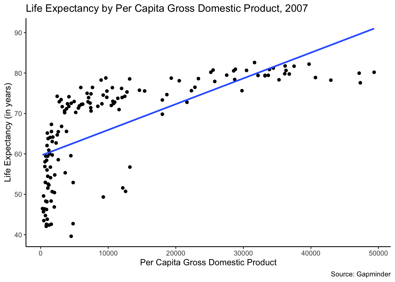
gapminder %>%
  filter(year == 2007) %>%
  ggplot(mapping = aes(x = pop, y = lifeExp)) +
  geom_point() +
  ggtitle("Life Expectancy by Per Capita Gross Domestic Product, 2007")+
  labs(x = "Population", y = "Life Expectancy (in years)", caption = "Source: Gapminder") +
  geom_smooth(method = lm, se = FALSE) +
  theme_classic()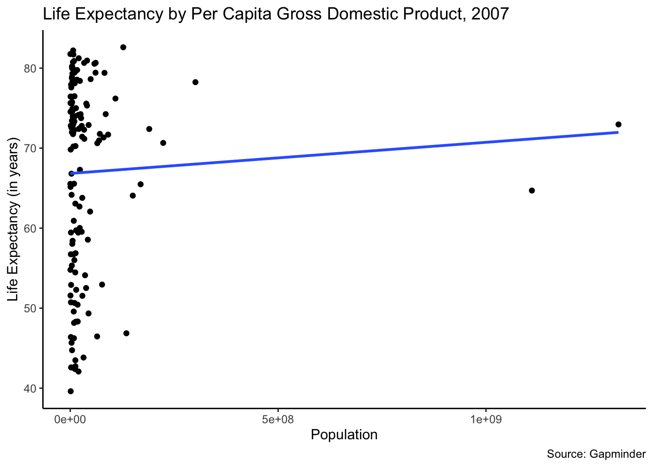
To make these easier to interpret, we can convert the x-axis variables with the arithmetic logs. We do this by using the log() function. This data transformation makes the shape of the data clearer and the shape of the data easier to interpret.
gapminder %>%
  filter(year == 2007) %>%
  ggplot(mapping = aes(x = log(gdpPercap), y = lifeExp)) +
  geom_point() +
  ggtitle("Life Expectancy by Per Capita Gross Domestic Product, 2007")+
  labs(x = "Per Capita Gross Domestic Product", y = "Life Expectancy (in years)", caption = "Source: Gapminder") +
  geom_smooth(method = lm, se = FALSE) +
  theme_classic()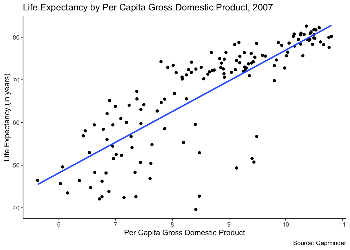
gapminder %>%
  filter(year == 2007) %>%
  ggplot(mapping = aes(x = log(pop), y = lifeExp)) +
  geom_point() +
  ggtitle("Life Expectancy by Per Capita Gross Domestic Product, 2007")+
  labs(x = "Population", y = "Life Expectancy (in years)", caption = "Source: Gapminder") +
  geom_smooth(method = lm, se = FALSE) +
  theme_classic()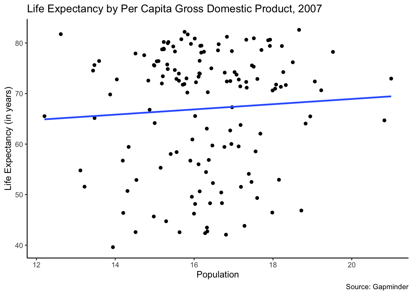
7.3.3 Example 3: Does Ethiopian’s national pride vary by education? (WVS)
With this example we will test the following hypothesis: The more education that an Ethiopian has, the higher will be their national pride.
We are taking this data from the WVS dataset. We managed the data above.
7.3.3.1 Run the chi-square test
Let’s run the chi-square test. We want to focus on the p-value. If it is smaller than .05, then we can reject the null hypothesis. We cannot reject the null hypothesis here, because the p-value is .317.
##
##  Pearson's Chi-squared test
##
## data:  ethiopia_small$Q254 and ethiopia_small$Q275R
## X-squared = 7.0376, df = 6, p-value = 0.3174
7.3.3.2 Examine your data in contingency tables
We can now look at the contingency table for this data. We will look at three tables. They show the following: 1. The observed data from the survey. 2. What we would expect to find if there was no relationship between the two variables. 3. The column percentages.
## Cross-Tabulation, Column Proportions
## Q254 * Q275R
## Data Frame: ethiopia_small
## Label: filelabel
##
##
## ------------------ ------- -------------- -------------- -------------- ---------------
##                      Q275R          Lower         Middle         Higher           Total
##               Q254
##         Very proud           683 ( 85.2%)   213 ( 88.4%)   162 ( 90.0%)   1058 ( 86.5%)
##        Quite proud            91 ( 11.3%)    21 (  8.7%)    14 (  7.8%)    126 ( 10.3%)
##     Not very proud            18 (  2.2%)     6 (  2.5%)     1 (  0.6%)     25 (  2.0%)
##   Not at all proud            10 (  1.2%)     1 (  0.4%)     3 (  1.7%)     14 (  1.1%)
##              Total           802 (100.0%)   241 (100.0%)   180 (100.0%)   1223 (100.0%)
## ------------------ ------- -------------- -------------- -------------- ---------------
##
## ----------------------------
##  Chi.squared   df   p.value
## ------------- ---- ---------
##    7.0376      6    0.3174
## ----------------------------## ethiopia_small$Q275R
## ethiopia_small$Q254 Lower Middle Higher
## Very proud 693.798855 208.48569 155.715454
## Quite proud 82.626329 24.82911 18.544563
## Not very proud 16.394113 4.92641 3.679477
## Not at all proud 9.180703 2.75879 2.0605077.3.3.3 Run the post-hoc test
Next, we will run the post-hoc test with the Bonferroni adjustment. As discussed in the PDS video, we have to adjust the p-value that we will use to test the null hypothesis. That adjustment is computed by taking the original p-value we use (.05) and dividing it by the number of comparisons (3 in this instance). This gives us .017. So, to be statistically significant a pair would need a p-value of .017 or lower.
In looking at the test below we focus on the raw.p number. In this case, none of the p-values are statistically significant.
We cannot reject the null hypothesis here. There is not a statistically significant relationship.
source('https://raw.githubusercontent.com/PassionDrivenStatistics/R/master/ChiSquarePostHoc.R')
chisq.post.hoc(national_pride$observed, control="bonferroni", popsInRows=FALSE)[,1:2]
## Adjusted p-values used the bonferroni method.## comparison raw.p
## 1 Lower vs. Middle 0.4884
## 2 Lower vs. Higher 0.2076
## 3 Middle vs. Higher 0.2585