9.1 Linear Regression

Linear regression is a core tool of social science. It is both powerful and robust. At its simplest, it is a fancier version of Pearson correlation. Because you can use multiple independent (explanatory) variables, it is a much more powerful tool. We will see that we can assess both the statistical significance of each independent (explanatory) variable using the t-test, and assess the power of the model as a whole, using R².

9.1.1 Simple Linear Regression

While you may have never used linear regression, you have seen the equation before beginning in algebra in middle school. All we are doing is looking to use the equation for a line:

\(y = mx + b\)

\(y\) = the predicted of the dependent variable
\(m\) = the the value of the independent variable
\(x\) = the predicted of the dependent variable
\(b\) = the error term

to predict the effects of one continuous variable on another. We will see that we can use categorical independent variables as well.

For more information on simple regression go to the Introduction to Modern Statistics textbook.

Example 1. For a first example, we will use Gapminder data. We will ask the question, does GDP per capita predict life expectancy for nations?

Let’s begin with a graph visualizing this data. A trend line that shows the regression model is included. The trend line and the data in the scatter plot shows a solid positive relationship between the two variables.

ggplot(gapminder) +
  aes(x = gdp_10_thou, y = lifeex_total) +
  geom_point() +
  labs(x="Log of GDP Per Capita in Thousands of US Dollars", y="Life Expectancy",
       title="Life Expectancy by GDP Per Capita in Thousands of US Dollars",
       subtitle="2007",
       caption="Data from Gapminder") +
  scale_x_log10() +
  geom_smooth(method = "lm", se = FALSE) +
  theme_bw()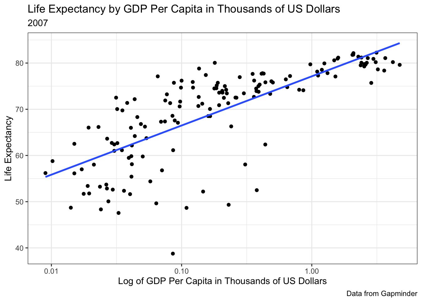

Next, we’ll run the regression model. The code below shows the basic format using the lm and summary commands.

nameOfObject <- lm(dependentVariable ~ independentVariable, data = dataset)
summary(nameOfObject)

Here is the code for our model:

life_exp_gdp_lm <- lm(lifeex_total ~ gdp_10_thou, data = gapminder)
summary(life_exp_gdp_lm)

## 
## Call:
## lm(formula = lifeex_total ~ gdp_10_thou, data = gapminder)
## 
## Residuals:
##     Min      1Q  Median      3Q     Max 
## -27.552  -5.174   2.272   6.477  13.216 
## 
## Coefficients:
##             Estimate Std. Error t value Pr(>|t|)    
## (Intercept)  65.8361     0.8039   81.89  < 2e-16 ***
## gdp_10_thou   5.5494     0.6817    8.14 1.54e-13 ***
## ---
## Signif. codes:  0 '***' 0.001 '**' 0.01 '*' 0.05 '.' 0.1 ' ' 1
## 
## Residual standard error: 8.318 on 147 degrees of freedom
##   (18 observations deleted due to missingness)
## Multiple R-squared:  0.3107, Adjusted R-squared:  0.306 
## F-statistic: 66.26 on 1 and 147 DF,  p-value: 1.542e-13

In interpreting our model we can want to look at three things:

the equation,
the t-test of the independent variable, and
the R² for the model as a whole.

The equation is:

\(Life Expectancy = 65.8 + 5.5 (GDP Per Capita)\)

65.8 and 5.5 come from the estimates in the model.

The t-test of the independent variable: The t-value is 8.14, and the probability is 1.54e-13, well below .05 needed to reject the null-hypothesis. The relationship is statistically significant. (A shorthand is if t > 2, then we have statistical significance and can reject the null hypothesis.)

R² is the percentage of the variance in the dependent variable explained by the model. For this simple regression model, R² = .31. This means that 31% of the variance in a nation’s life expectancy is explained by GDP per capita.

Example 2

For a second example, we will use data on U.S. governor public opinion gathered for late-219. We will ask the question, Does political party affiliation impact the public’s approval of U.S. governors?

Let’s begin with a graph visualizing this data. Because the independent (explanatory) variable is categorical, we will look at a box plot. There does appear to be a difference based on party, with Republican governors showing higher approval ratings than Democratic governors.

ggplot(us_states_2019) +
  aes(x = party, y = govPopularity) +
  geom_boxplot() +
  labs(x="Political Party", y="Percent Support for Governor",
       title="Gubernatorial Popular Support by Political Party",
       subtitle="late 2019",
       caption="Support Data from Politico") +
  scale_x_discrete(labels = c('Democrats','Republicans')) +
  theme_minimal()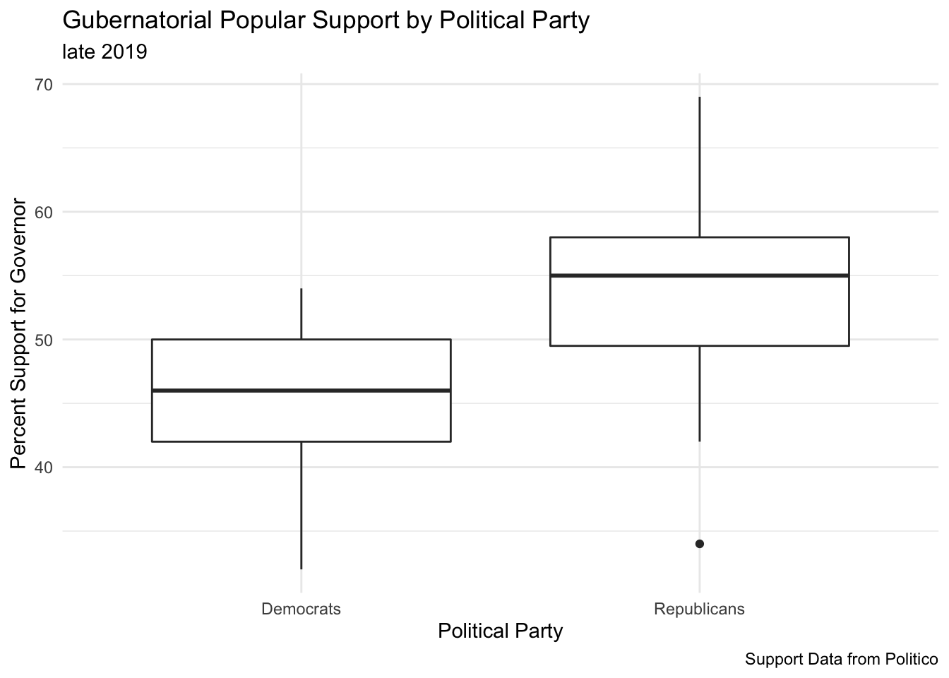

Now let’s run our model. The categorical independent variable is known as a dummy variable in regression analysis. R knows how to handle such variables. As we will see in the output below, in producing results, one category is excluded. Democratic governors are excluded from the results. We will interpret the party variable to mean: how much difference does it make if a governor is a Republican?

gov_party_lm <- lm(formula = govPopularity ~ party , data = us_states_2019) 
summary(gov_party_lm)

## 
## Call:
## lm(formula = govPopularity ~ party, data = us_states_2019)
## 
## Residuals:
##      Min       1Q   Median       3Q      Max 
## -20.0741  -3.1304   0.8977   3.9259  14.9259 
## 
## Coefficients:
##                 Estimate Std. Error t value Pr(>|t|)    
## (Intercept)       45.130      1.592  28.346  < 2e-16 ***
## partyrepublican    8.944      2.167   4.128 0.000145 ***
## ---
## Signif. codes:  0 '***' 0.001 '**' 0.01 '*' 0.05 '.' 0.1 ' ' 1
## 
## Residual standard error: 7.636 on 48 degrees of freedom
## Multiple R-squared:  0.262,  Adjusted R-squared:  0.2466 
## F-statistic: 17.04 on 1 and 48 DF,  p-value: 0.0001451

In interpreting our model we want to look at three things: the equation, the t-test of the independent variable, and the R² for the model as a whole.

The equation is:

\(GovernorApproval = 45.1 + 8.9 (RepublicanParty)\)

45.1 and 8.9 come from the estimates in the model.

The t-test of the independent variable: The t-value is 4.1, and the probability is 0.000145, well below .05. We reject the null-hypothesis. The relationship is statistically significant. (A shorthand is if t > 2, then we have statistical significance and can reject the null hypothesis.)

R² is the percentage of the variance in the dependent variable explained by the model. For this simple regression model, R² = .26. This means that 26% of the variance in a nation’s life expectancy is explained by GDP per capita.

9.1.2 Multiple Linear Regression

Regression is very flexible and allows for several, even many, independent (explanatory) variables. The formula is expanded to: \(y = mx + b1 + b2 + . . .\) Expanding on the earlier examples, we will look at multiple regression.

To create the models in R we will again use the lm and summary commands.

nameOfObject <- lm(dependentVariable ~ independentVariable1 + independentVariable2 + independentVariable3, data = dataset)
(summary(nameOfObject))

For more information on multiple regression go to the Introduction to Modern Statistics textbook.

Example 1. In our multiple regression model attempting to explain life expectancy, we will add the following independent (explanatory) variable:

GDP per capita
whether the nation is an OECD country
the literacy rate
the polity score of how democratic a nation is
the population of a nation
the Gini index measuring economic inequality

life_exp_multi_lm <- lm(lifeex_total ~ oecd + literacy + polity + gdp_10_thou + pop_total + gini10, data = gapminder)
summary(life_exp_multi_lm)

## 
## Call:
## lm(formula = lifeex_total ~ oecd + literacy + polity + gdp_10_thou + 
##     pop_total + gini10, data = gapminder)
## 
## Residuals:
##      Min       1Q   Median       3Q      Max 
## -20.0660  -2.8923   0.2795   4.4349  17.7811 
## 
## Coefficients:
##                        Estimate Std. Error t value Pr(>|t|)    
## (Intercept)           53.516935   4.022880  13.303  < 2e-16 ***
## oecdOECD Member state  0.122392   2.742540   0.045  0.96448    
## literacy               0.254028   0.032710   7.766 3.27e-12 ***
## polity                 0.251060   0.121566   2.065  0.04109 *  
## gdp_10_thou            2.246338   1.084924   2.071  0.04059 *  
## pop_total              0.003937   0.003665   1.074  0.28492    
## gini10                -0.197570   0.074853  -2.639  0.00943 ** 
## ---
## Signif. codes:  0 '***' 0.001 '**' 0.01 '*' 0.05 '.' 0.1 ' ' 1
## 
## Residual standard error: 6.738 on 118 degrees of freedom
##   (42 observations deleted due to missingness)
## Multiple R-squared:  0.5847, Adjusted R-squared:  0.5636 
## F-statistic: 27.69 on 6 and 118 DF,  p-value: < 2.2e-16

In interpreting our model we want to look at three things:

the equation,
the t-test of the independent variable, and
the R² for the model as a whole.

The equation is:

\(Life Expectancy = 53.5 + .12 (OECD) + .25 (Literacy) + .25 (Polity) + 2.2 (GDP) + .003 (Pop) -.19 (Gini)\)

The t-test of the independent variable: Examining the t-values and probability tests, we see that literacy, the polity score, GDP per capita, and the Gini Index are all statistically significant. (A shorthand is if t > 2, then we have statistical significance and can reject the null hypothesis.)

R² is the percentage of the variance in the dependent variable explained by the model. For this simple regression model, R² = .58. This means that 58% of the variance in a nation’s life expectancy is explained by our model.

Example 2.

In our multiple regression model attempting to explain public approval of U.S. governors, we will add the following independent (explanatory) variable:

gender of the governor
how long the governor has been in office
the governor’s political party
the state’s population
the state’s unemployment rate

gov_all_lm <- lm(formula = govPopularity ~ gender + inauguration + party + adjPop + unempRate, data = us_states_2019) 
summary(gov_all_lm)

## 
## Call:
## lm(formula = govPopularity ~ gender + inauguration + party + 
##     adjPop + unempRate, data = us_states_2019)
## 
## Residuals:
##      Min       1Q   Median       3Q      Max 
## -19.4390  -3.4287   0.6585   3.7422  14.5988 
## 
## Coefficients:
##                   Estimate Std. Error t value Pr(>|t|)   
## (Intercept)      15.334774 902.372029   0.017  0.98652   
## gendermale        6.569479   2.967604   2.214  0.03208 * 
## inauguration      0.015431   0.446923   0.035  0.97261   
## partyrepublican   7.609969   2.162181   3.520  0.00102 **
## adjPop           -0.002391   0.014985  -0.160  0.87397   
## unempRate        -1.645842   1.309592  -1.257  0.21547   
## ---
## Signif. codes:  0 '***' 0.001 '**' 0.01 '*' 0.05 '.' 0.1 ' ' 1
## 
## Residual standard error: 7.337 on 44 degrees of freedom
## Multiple R-squared:  0.3754, Adjusted R-squared:  0.3044 
## F-statistic: 5.288 on 5 and 44 DF,  p-value: 0.0006883

In interpreting our model, we can want to look at three things:

the equation,
the t-test of the independent variable, and
the R² for the model as a whole.

The equation is:

\(Governor Approval = 53.5 + 6.6 (Male) + .01 (Months in Office) + 7.6 (Republican) - .002 (Pop) - 1.65 (Unemployment)\)

The t-test of the independent variable: Examining the t-values and probability tests, we see that only gender and party are statistically significant. (A shorthand is if t > 2, then we have statistical significance and can reject the null hypothesis.)

R² is the percentage of the variance in the dependent variable explained by the model. For this simple regression model, R² = .37. This means that 37% of the variance in a governor’s public approval rating is explained by our model.